Residual Network

This post is mainly based on

• Deep Residual Learning for Image Recognition, CVPR 2016
• Residual networks behave like ensembles of relatively shallow networks, NIPS 2016
• Visualizing the Loss Landscape of Neural Nets, NIPS 2018

Residual network is first introduced by He’s team in 2015 and is one of the most influential paper in deep learning. Residual connection enabled training of very deep network (e.g., 152 layers on ImageNet or 1202 layers on CIFAR-10) and beat state of art benchmark on classification problem by a large margin.

Efforts have been made to understand why network with residual connections can be efficiently trained. Both the 2016 and 2018 paper are empirical studies. The 2016 paper show that residual network can be decomposed into an ensemble of shallow networks. The effective paths in residual networks are shorter, possibly makes the optimization problem easier. The 2018 paper visualized loss surfaces of network with and w/o residual connections and their result suggest that residual connections make the loss landscape significantly smoother. ow

Residual Connection

Multiple research have shown that deep network leads to better performance in CV tasks, due to deep network can approximate more complex non-linear function and it naturally integrate low/mid/high-level features. However, deep networks are very hard to optimize. Deep networks suffer from vanishing/exploding gradient problem, which can be solve with batch normalization. In previous post, we found that batch normalization can effectively prevent loss function divergence at the beginning of the optimization. However, the authors observe that even if deep network can converge, it typically suffers from the degradation problem.

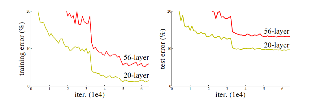Training error (left) and test error (right) of 20-layer and 56-layer networks w/o residual connection on CIFAR-10

The above figure shows the degradation problem: adding more layers to a suitably deep model leads to higher training error. Note that this is not a overfitting problem. A deep network should be able to reach at least same training error as its shallow counterpart. This can be achieved by copying its shallow counterpart and initialize the excessive layers to the identity mapping. This observation indicated that degradation problem was caused by optimization.

Zero Mapping vs Identity Mapping

The authors points out that feedforward network naturally biased toward learning the zero mapping due to random initialization (and regularization). If a shallow network is optimal, then degradation problem is caused by optimizer have difficulties in learning the identity mappings. The idea of residual connection is bias the function between layers toward the identity mapping.

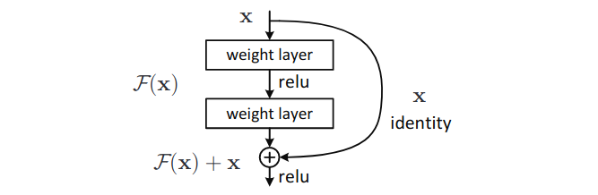
Assume $H(x)$ is the optimal function and $H(x)$ is close to the identity mapping. Residual connection reformulate the problem to learn a small perturbation $F(x) = H(x) - x$. The perturbation naturally biased toward the zero mapping, which makes the optimization easier.

Performance

Before ResNet, the state of art architecture is VGG-16, which can achieve 9.33% top 5 testing error on an ImageNet benchmark. ResNet-152 is able to reach testing error of 5.71%. The more Remarkable result is that ResNet-152 is able to reach this accuracy with fewer parameters (ResNet-152 has about 60M parameters, VGG-16 has around 138 million parameters) and lower computation complexity (ResNet-152 has 11.3 billion FLOPs complexity, VGG-16 has 15.3 billion FLOPs complexity).

This paper also established a bunch of techniques that are specific to CV problems, such as bottleneck layer (1x1 conv to reduce number of parameter in 3x3 conv) and downsampling conv with stride of 2 (instead of pooling layers). Interested reader please refer to the paper for details.

Note that residual network is different from boosting as explained in Learning Deep ResNet Blocks Sequentially using Boosting Theory, ICML 2018

Ensemble of Shallow Networks

The motivation of the original ResNet is to biased the initial state of network to identity mapping. The authors believes that learning a skip connection on top of the identity mapping is much easier than learning an identity mapping from a scratch. The 2016 paper proposed another interpretation: residual network can be viewed as an explicit collection of paths. Paths behave like model ensemble. Most of those paths are considerably shorted than the nominal network depth, possibly makes the optimization problem less challenging.

Consider the representation of residual connection where $y_{i-1}$ is the output from (i-1)-th layer and $f_i$ is the mapping of residual connection:

\[y_i = f_i(y_{i−1}) + y_{i−1}\]

We can rewrite a 3-layer network as

\[\begin{align} y_3 &= f_3(y_2) + y_2 \\ y_3 &= f_3[f_2(y_1) + y_1] + f_2(y_1) + y_1 \\ y_3 &= f_3\{f_2[f_1(x) + x] + [f_1(x) + x]\} + f_2[f_1(x) + x] + f_1(x) + x \end{align}\]

Or equivalently,

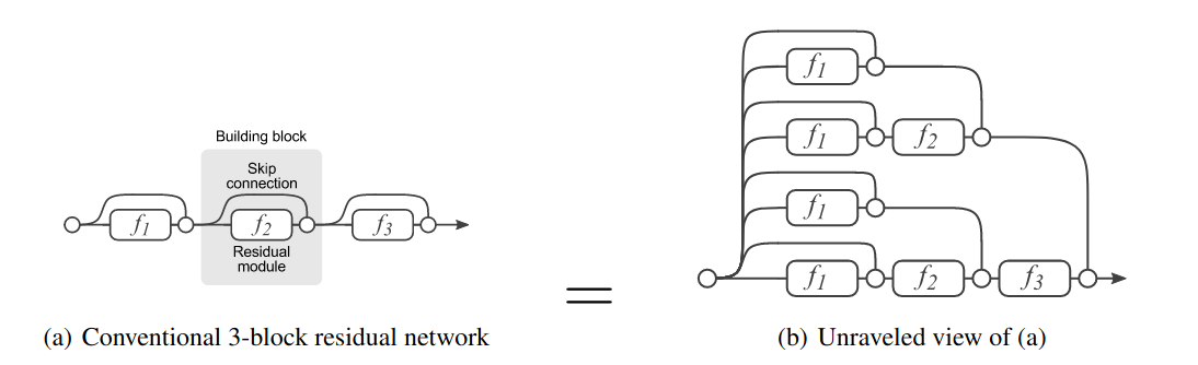
The above graph shows that data flows though many paths to generate $y$ and there one can show that are $2^n$ paths from input to output. In feedforeward network, each layer strictly receive input from previous layer and there is only one path available. In ResNet, each layer receive input from $2^{n-1}$ different paths. Therefore delete one layer (and the corresponding paths to that layer) have limited impact on the performance of the network. This is the why stochastic depth could work in training.

Ensemble-like behavior

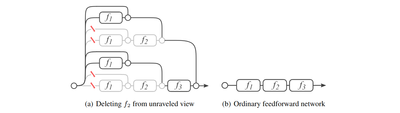
The authors argue that the collection of paths behave like ensemble in predicting and tested their hypothesis by the following experiments: train the ResNet with normal procedure (no layer removal in training). In testing, remove individual layers and check for the impact on performance. The removal individual layers can be express as:

\[y_i = y_{i−1} + f_i(y_{i−1}) \Longrightarrow y_i = y_{i−1}\]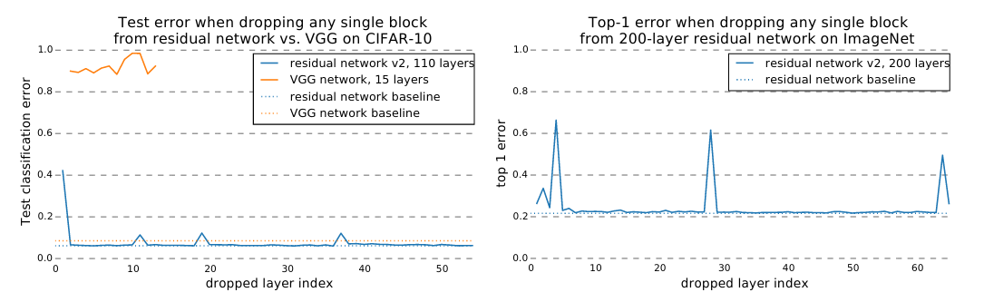

Left: deleting individual layers from VGG-15 and ResNet on CIFAR-10; right: deleting individual layers from ResNet on ImageNet

Removing any layer from VGG render the model useless. However, removing most of the layers from ResNet have limited impact on the network; removing downsampling modules has a slightly higher impact. The result suggests that the collection of paths show ensemble-like behavior: the collection of paths all contribute to the prediction and paths do not strongly depend on each other.

Distribution of path lengths

The path length distribution of ResNet as shown in (a). For a residual network with 54 modules, more than 95% of paths go through 19 to 35 modules. Due the topology of the network, path length follows a Binomial distribution. For example:

• There is one path that go through non of the $f_i$ and one path that go through all the $f_i$
• There are $n$ path that go through 1 $f_i$ and $n$ path that go through $n-1$ the $f_i$
• The mean path length is $n/2$

Gradient flow through individual path is also investigated as shown in (b): To sample a path of length k, we first feed a batch forward through the whole network. During the backward pass, we randomly sample k residual blocks. For those k blocks, we only propagate through the residual module; for the remaining n − k blocks, we only propagate through the skip connection. The result suggests that gradient can easily follow through short path.

Gradient flow through one path is different from gradient contribution by an individual layer. The automatic differentiation. (AD) relays on chain rule: although magnitude of gradient on deeper layer is low, these nodes got multiplied many times in the computation graph of AD.

The authors measure the total gradient magnitude contributed by paths of each length as shown in (c): we multiply the frequency of each path length with the expected gradient magnitude. The result suggests that almost all of the gradient updates during training come from paths between 5 and 17 modules long. These are the effective paths, even though they constitute only 0.45% of all paths through this network. Moreover, in comparison to the total length of the network, the effective paths are relatively shallow.

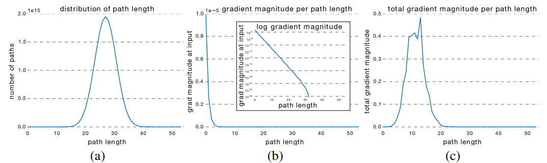_(a) path length distribution for a residual network with 54 modules; _

Smoother Optimization Landscape

Training neural networks requires minimizing a non-convex loss function and the architecture of the network influence the shape of the loss function. The 2018 paper took a different path in explaining why ResNet makes optimization easier: they focus on the visualization of the optimization landscape and show that the residual connection yields a smoother optimization landscape.

These plots are generated by the following procedure: They optimize models using SGD on CIFAR-10 dataset until convergence and then use local minima obtained from the optimization as the center of xy-plane. Loss surface is visualized by Random Direction + Filter-Wise Normalization. I was initially plan to write about this method but it appears that the topic itself is worth discussing in a separate post. If you are interested in how to visualize a high dimensional loss surface in 2D, and it implications on optimization, please read this post. Results are as follow:

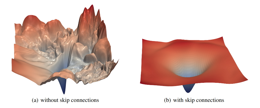Surface plots of ResNet-56 with and without residual connection

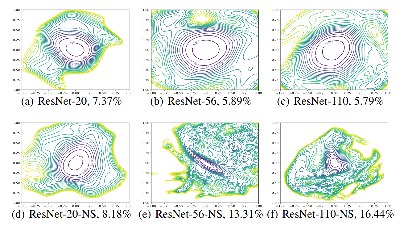Contour plots of ResNet-20/56/110 with and without residual connection (NS stands for “no-skip”)

There are two takeaways from the above result

• For network without residual connection, depth has a dramatic effect on the loss surfaces. As network depth increases beyond 20, the loss surface transform from convex to highly non-convex. Optimization on highly non-convex surface likely lead to Shattered Gradients mentioned in The Shattered Gradients Problem: If resnets are the answer, then what is the question?, PMLR 2017.
• Residual connection has a dramatic effect on the loss surfaces. Residual connection prevent the loss surface from transforming into highly non-convex shape.

Afterthoughts

Despite ResNet was invented in 2016, the reason why it can help optimization is still not well understood and most of the analysis are based on empirical studies. If you are interested in a theoretically analysis, this paper on a 2-layer Conv ResNet, may worth a reading.