Batch Normalization
This post is mainly based on
- Batch Normalization: Accelerating Deep Network Training by Reducing Internal Covariate Shift, ICML 2015
- Understanding Batch Normalization, NIPS 2018
- How Does Batch Normalization Help Optimization?, NIPS 2018
Batch Normalization is implemented as a layer and is typically added after Conv-layer or FC-layer and before activation layer. The idea is very simple: we want unit gaussian distribution output at every feature and every layer of the network. So we just normalize the output at batch level:
\[x \xrightarrow{\text{previous layer}} y \xrightarrow{\text{standardize}} \hat{y} \xrightarrow{\text{shift and scale}} z\]Consider a mini-batch input $B = {y_1, …, y_m}$, where $y = Wx$ (both Conv-layer or FC-layer can be written as $y = Wx$). Batch Normalization produces output ${z_i = \operatorname{BN}_{\gamma, \beta}(y_i)}$. It have two trainable parameters: $\gamma, \beta$
Algorithm (following notations from the third paper)
- compute mini-batch mean: $\mu_B = \frac{1}{m} \sum_i y_i$
- compute mini-batch variance: $\sigma_B^2 = \frac{1}{m} \sum_i (y_i - \mu_B)^2$
- compute normalize $y$: $\hat{y}_i = \frac{y_i - \mu_B}{ \sqrt{\sigma_B^2 + \varepsilon}}$
- scale and shift $\hat{y}$: $z_i = \gamma \hat{y}_i + \beta$
The original batch normalization paper was published in 2015. It allowed faster training of network and achieve lower validation error. The authors believe that the success was due to batch normalization reduced internal covariate shift.
Two paper published in 2018 further investigate this topic and argues that internal covariate shift only has minor effects. One paper found that BN effectively controls the magnitude of gradient. Thus, the network can be trained with higher learning rates without divergence. The concluded that the better generalization accuracy was due to higher learning rates which allows the optimizer to escape sharp local minima. The second paper analyze the loss shape and found that batch normalization makes the optimization landscape significantly smoother, which enables faster and more effective optimization. They analyzed the effect of BatchNorm on the Lipschitzness of the loss, and proved that $\frac{\partial L}{\partial \hat{y}}$ for network with batch normalization is bounded by a shifted and rescaled $\frac{\partial L}{\partial y}$ for network without batch normalization.
The Original Batch Normalization Paper
They applied Batch Normalization to the best-performing ImageNet classification network, and showed that network with batch normalization can reach same accuracy using only 7% of the training steps, and network with batch normalization achieved validation accuracy exceed network without batch normalization by a substantial margin.
Internal Covariate Shift
The authors noted that durning training, the distribution of each layer’s inputs changes due to the parameters of the previous layers change. Consider network learns a conditional distribution $P(y|x)$ and output correct $P(x, y) = P(y|x)P(x)$. If the input distribution changes to $P’(x)$, then $P(y|x)P’(x)$ no longer yield the correct distribution. This slows down the training by requiring lower learning rates and careful parameter initialization. They posit that the problem can be solved by normalizing layer output, and this leads to the idea of batch normalization.
Batch Normalization
Batch normalization is easily differentiable since only addition and multiplication is involved.
During training, $\mu_B, \sigma_B$ for each batch is different and is calculated on the fly. During testing, batch normalization aim to avoid the randomness created by averaging over batch data, so each batch will be normalized by a fixed $\mu_B, \sigma_B$. This fixed $\mu_B, \sigma_B$ can be computed by keeping a exponential moving average of the mean and variance during training and stored as part of the layer’s state.
You may be curious about why batch normalization have a shift and scale step $\hat{y}$: $z_i = \gamma \hat{y}_i + \beta$. Without this step, the output from batch normalization layer is always a standard normal distribution, which could be suboptimal for the network. For example, optimization could decided that the output distribution should be, say $N(0.5,0.2)$, before the $\tanh$ activation. Without the scale and shifting step, the output is always $N(0,1)$. The scale and shifting parameters $\gamma, \beta$ are in the same computation graph and can also be learned by automatic differentiation.
Advantage
- Allow higher learning rates
- Weak regularization effect
Batch normalization allows higher learning rates, due to:
\[\frac{\partial BN( (aW)x )}{\partial x} = \frac{\partial BN(Wx)}{\partial x}\] \[\frac{\partial BN( (aW)x )}{\partial(aW)} = \frac{1}{a} \frac{\partial BN(Wx)}{\partial W}\]The first equation shows that gradient w.r.t $x$ (gradient flow through to shallower layers) is not affected by the scale of the weight parameter. The second equation shows that the gradient on weight is reduced for larger weight. Hence, higher learning rate $a$ is possible.
For the weak regularization effect, due to normalization factor is calculate batch, each input $x$ is slightly perturbed and stochastic, which could act as a weak regularizer.
Understanding Batch Normalization (BN)
The authors of this paper believed that Internal Covariate Shift is not the main reason behind the success of batch normalization: We do not claim that internal covariate shift does not exist, but we believe that the success of BN can be explained without it. We argue that a good reason to doubt that the primary benefit of BN is eliminating internal covariate shift. They took an empirical approach: comparing behavior of networks with and without BN on an interval of viable learning rates. Their conclusion: BN primarily enables training with larger learning rates, which is the cause for faster convergence and better generalization.
Disentangling Benefits of BN
Without BN, the initial learning rate of Resnet needs to be decreased to $\alpha = 0.0001$ for convergence and training takes roughly 2400 epochs. Benefits of BN are:
- Faster convergence
- Higher accuracy
- Enable higher learning rates
Goal: disentangle how these benefits are related
Approach
- Train network with BN and w/o at same learning rate and analyze the convergence
- Train network with BN at lower and higher learning rate and analyze the convergence
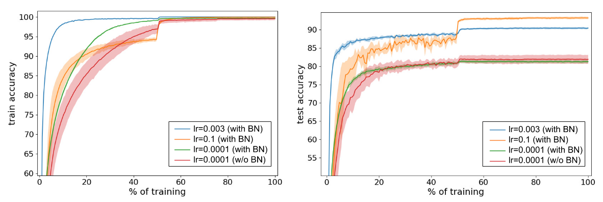 Network: 110-layer Resnet. All results are averaged over five runs with std shown as shaded region around mean
Comparing testing accuracy of lr = 0.0001 with BN and lr = 0.0001 w/o BN, we found that at same learning rate, network with BN performs worse that network w/o BN. Comparing lr = 0.0001 with BN, lr = 0.003 with BN and lr = 0.1 with BN, we found that higher learning rate result in better testing accuracy. The authors argues that higher learning rate may help bypass sharp local minima, which was discussed in [TBD: this post].
BN Prevents Divergence
Previously the author mentioned that without BN, the network cannot be trained with higher learning rate due to divergence, which typically happens in the first few mini-batches. Therefore they analyzed gradients at initialization:
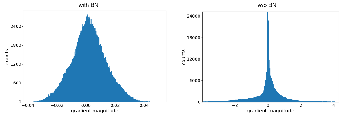
Histograms over the gradients at initialization for (midpoint) layer 55 of a network
Without BN, gradients distributions are heavy tailed, and are almost 100x larger than network with BN.
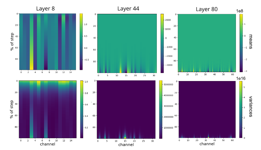 Heatmap of channel means and variances, for channels in layer-8, layer-44 and layer-80 in network w/o BN, during a diverging gradient update. y-axis: percentage of the gradient update has been applied.
This graph may be a bit confusion. The graph is a heatmap of activation outputs. The graph is generated at the step when the loss function explode. Parameters are updated sequentially and the y-axis indicated what % of parameters in the network are updated. The channel’s output exploded to 1e8 at deeper layers (layer-80) at the end of this update (y-axis > 80%). This showed that during an early on-set of divergence, a small subset of activations (typically in deep layer) “explode.
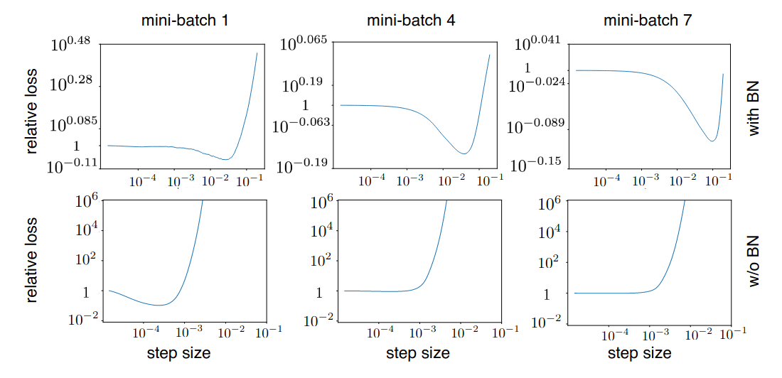 Relative loss over a mini-batch as a function of the step-size/learn rate.
Throughout all cases the network with BN is far more forgiving and the loss is well behaved over larger ranges of learn rate.
Random initialization lead to divergence
This is an interesting section where the authors argue that gradient explosion in a deep networks, w/o BN, with random initialization, is almost guaranteed. Which contradict with our previous understanding of Xavier initialization, which is discussed in this post. They abstract neural network into a sequence of linear transformation $y = A_t A_2 A_1 x$. They argue that if $A_i$ are random matrices, as $t \uparrow$, the matrix product will have some high singular values with high probability. If $x$ took the direction close the one of its right singular vectors, $y$ are likely explode and result in loss divergence.
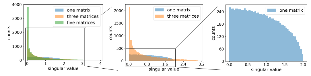 Distributions of singular values of product of independent matrices. The matrices have dimension N=1000 and all entries independently drawn from a standard Gaussian distribution. Experiments are repeated ten times. Plot on the right are “zoom in” of graph on the left.
Distribution of singular values becomes more heavy-tailed as more matrices are multiplied, which represents a deeper linear network.
How Does Batch Normalization Help Optimization
Compared to the second paper, the authors of the third paper analyzed BN in a more theoretical approach. They argue that Internal Covariate Shift has little to do with the success of BatchNorm. They found that BN induced a significantly smoother optimization landscape and this smoothness result in a more predictive and stable behavior of the gradients, allowing for faster training.
Isolating the effects of Internal Covariate Shift
They propose two experiments. In the first experiment, they train networks with random noise injected after BN layers. The noise are sampled from a time varying, non standard Guassian distribution, which produces a severe covariate shift that skews activations at every time step.
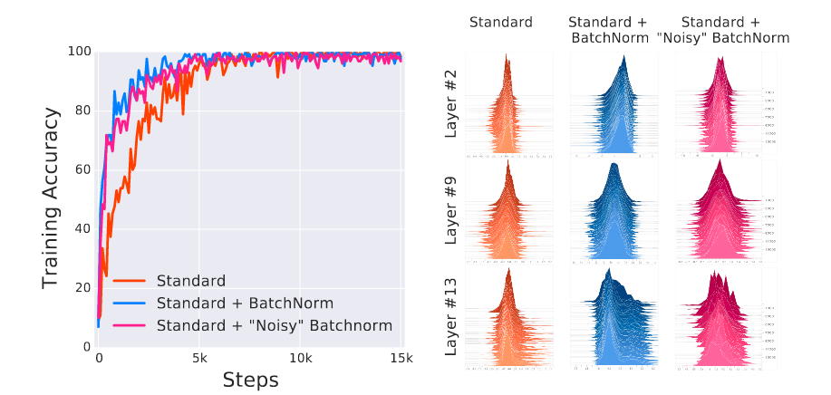 Left: convergence of VGG networks; right: distributions of activations of layer-2, 9 and 13 for VGG networks
On the left plot, distributions of Standard +"Noisy" BatchNorm are less stable than Standard across time (front to back). However, Standard +"Noisy" BatchNorm still achieved faster convergence compared to Standard.
In the second experiment, they measure the difference between gradient of a normal gradient step $G$ and gradient of a hypothetical step if the same data $x$ is used again $G’$. They argue that different between $G$ and $G’$ can quantify Internal Covariate Shift.
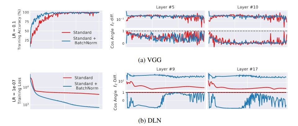 DLN: deep linear network
Their measure of Internal Covariate Shift for DLN with BN is surprisingly higher. The result showed that BN might not even reduce the internal covariate shift.
Optimization Landscape
They use Lipschitz in their analysis. Note that $f$ is L-Lipschitz if
\[|f (x_1) − f (x_2)| \leq L‖x_1 − x_2‖, \forall x_1, x_2\]In other words, if $f$ is L-Lipschitz, it cannot change too fast and its gradient is bounded by $L$.
The authors prove that BN improvement in the Lipschitzness of the loss function. After all, improved Lipschitzness of the gradients gives us confidence that when we take a larger step in a direction of a computed gradient, this gradient direction remains a fairly accurate estimate of the actual gradient direction after taking that step. Therefore, higher learning rate is more stable for network with BN. The main result is:
\[\left\|\nabla_{\boldsymbol{y}_{j}} \widehat{\mathcal{L}}\right\|^{2} \leq \frac{\gamma^{2}}{\sigma_{j}^{2}}\left(\left\|\nabla_{\boldsymbol{y}_{j}} \mathcal{L}\right\|^{2}-\frac{1}{m}\left\langle\mathbf{1}, \nabla_{\boldsymbol{y}_{j}} \mathcal{L}\right\rangle^{2}-\frac{1}{m}\left\langle\nabla_{\boldsymbol{y}_{j}} \mathcal{L}, \hat{\boldsymbol{y}}_{j}\right\rangle^{2}\right)\]where $\mathcal{L}$ is the loss for network w/o BN and $\hat{\mathcal{L}}$ is the loss for network with BN. $y = Wx$, output of linear layer. $\sigma_j$ is the standard deviation over a batch of outputs $y_j \in \mathbb{R}^m$. $\gamma$ is the scaling factor of BN.
The authors note that both \(\left\langle\mathbf{1}, \nabla_{\boldsymbol{y}_{j}} \mathcal{L}\right\rangle^{2}\) and \(\left\langle\nabla_{\boldsymbol{y}_{j}} \mathcal{L}, \hat{\boldsymbol{y}}_{j}\right\rangle^{2}\) should be large, so \(\left\|\nabla_{\boldsymbol{y}_{j}} \mathcal{L}\right\|^{2}\) is subtracted by two large numbers. In addition, $\sigma_j$ tends to be large in practice, making the multiplicative term small. Therefore, BN effectively improves the gradient bound of loss function. Please refer to the paper for more details.
In the experimental study, the authors visualize the smoothness of the loss function and the result shows that BN improve the smoothness of the loss function.
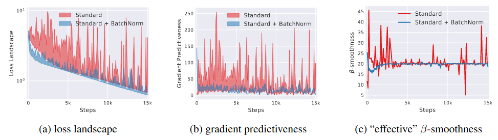 Optimization landscape of VGG networks. At a particular training step, we measure (a) the variation (shaded region) in loss (b) L2 changes in the gradient as we move in the gradient direction. (c) The “effective” $\beta$-smoothness as the maximum difference (in L2 norm) in gradient over distance moved in that direction.