Neural Loss Visualization
This post is mainly based on
- Visualizing the Loss Landscape of Neural Nets, NIPS 2018
- Tom Goldstein’s seminar (Tom Goldstein is one of the authors and this seminar is really good)
- The Shattered Gradients Problem: If resnets are the answer, then what is the question?, PMLR 2017
Neural network contains millions of parameters and its loss function is high dimensional. How to visualize a high dimensional loss surface in a low dimension space is the main problem. Existing visualization techniques includes: 1-Dimensional Linear Interpolation and Contour Plots & Random Directions.
Visualization methods
1-Dimensional Linear Interpolation
Randomly sample two parameters $\theta, \theta’$ and parameterize this direction $\theta(\alpha) = (1-\alpha)\theta + \alpha\theta’ $. The loss function can be visualized on a 1-D plot where the x-axis is $\theta(\alpha)$. This is an intuitive way to visualize the sharpness / rate of change of a function. However, the authors mentioned that it is difficult to visualize non-convexities on 1D plot.
Contour Plots & Random Directions
Randomly choose a center point $\theta^*$ and 2 direction $\delta, \eta$. The loss surface can be visualized as \(f(\alpha, \beta) = L(\theta^* + \alpha\delta + \beta\eta)\). However, computational cost of this method is high.
Besides there are some common problems faced by the above two methods. The first problem is batch normalization (BN). BN normalized the output following a linear layer. Therefore, scaling the weight parameter (due to we pick one direction) may induce very small changes on the output. The second problem is scaling effect: different parameters may have different scales. Perturbing one parameter by 0.01 may induce much greater impact on the output than perturbing other parameters by 0.01. This also make comparing two networks different: what scale should be used as the “unit perturbation”?
Filter-Wise Normalization
To solve the scaling effect, the authors proposed Filter-Wise Normalization. The idea is to normalize each parameter by the scale of its filter. The procedure is as follow:
- Step 1: obtain a random direction
- Sample a random Gaussian vector $d$ with dimensions compatible with $\theta$
- Step 2: normalize $d$ with the scale of filter
- \[d_{i,j} = \frac{ || \theta_{i,j} ||_F }{ ||d_{i,j}||_F } d_{i,j}\]
- i,j represents the j-th filter of the i-th layer
- \(\| \cdot \|_F\) stands for frobenius norm of a matrix
- \(\| \theta_{i,j} \|_F\) compute the average scale of the j-th filter of i-th layer
Does this really visualizing convexity?
With Random Directions method, if the network has $n$ parameters, we are dramatically reducing the dimension of loss function: from $n$ to 2. Can such visualizing reliably preserve the convexity in high dimensional space? I think the answer is mostly yes. The authors provided their answer using eigenvalues of the Hessian and provided some visualizations. I want to discuss this from another view: the space of loss function requires $n$ vectors to span. If the surface of loss function is highly non-convex, then the surface of loss on 2 random sampled direction is also non-convex with high probability. I think the fact that we are doing the random sampling makes the surface generated more representative. In the seminar, the author discussed previous research that performs dimension reduction using the gradient direction and produce poor result. If you are interested in this topic, I highly recommend you to watch this seminar.
Experiments
Depth
For network without residual connection, depth has a dramatic effect on the loss surfaces
- As network depth increases beyond 20, the loss surface transform from convex to highly non-convex
- Optimization on highly non-convex surface likely lead to Shattered Gradients mentioned in this paper
- Shattered Gradients are a sequence of gradients which have very low auto-correlation. This may be caused by walking on highly non-convex surface
- Under shattered Gradients, gradient descent possible behave more like random walk, rendering optimization ineffective
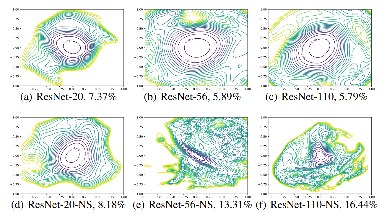 Contour plots of ResNet-20/56/110 with and without residual connection (NS stands for “no-skip”). Test error is reported below each figure.
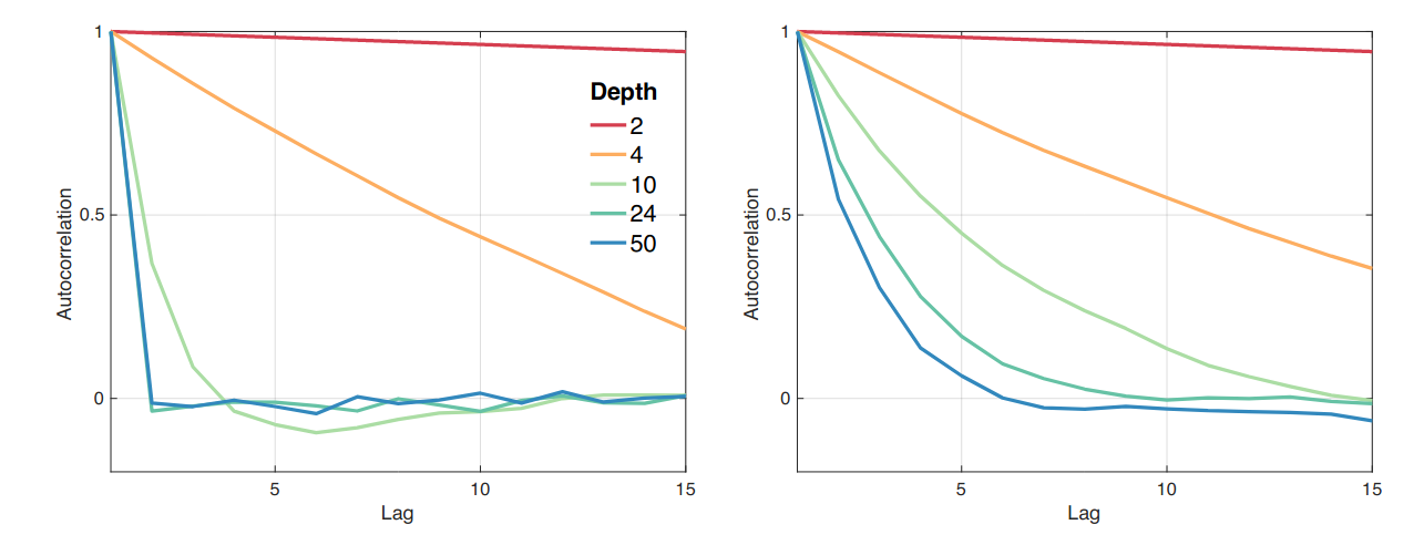 Left: Autocorrelation Function (ACF) of feedforward network with different depth; right: ACF of ResNets with different depth; Results are average over 20 runs
Residual connection
Residual connection has a dramatic effect on the loss surfaces. Residual connection prevent the loss surface from transforming into highly non-convex shape
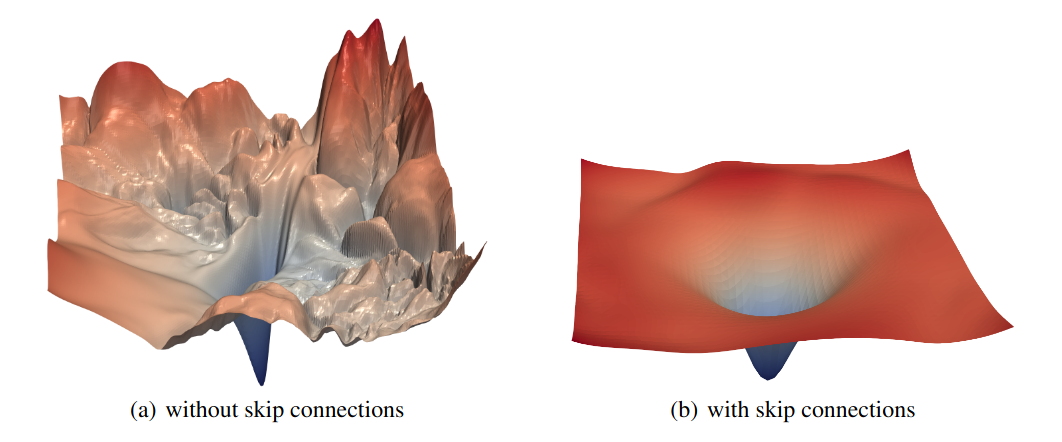 Surface plots of ResNet-56 with and without residual connection
Wide network
Wide network make the optimization landscape smoother.
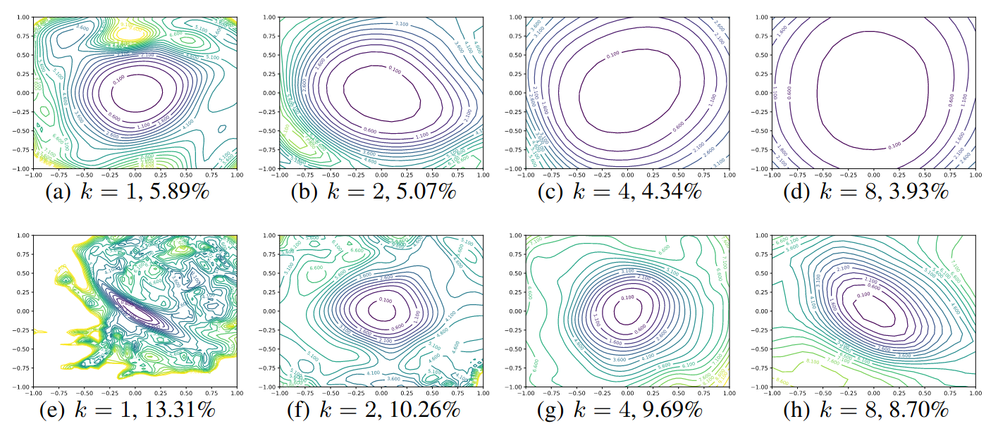 Contour plots of Wide-ResNet-56 on CIFAR-10 both with shortcut connections (top) and without (bottom). The label k = 2 means twice as many filters per layer. Test error is reported below each figure.
Sharpness of Minimizer
Authors mentioned that that sharpness minimizer correlates extremely well with testing error, as shown in the test error reported below each figure. Visually flatter minimizers consistently correspond to lower test error. Chaotic landscapes (deep networks without skip connections) result in worse training and test error, while more convex landscapes have lower error values. The most convex landscapes (Wide-ResNets) generalize the best of all. We will discuss a popular hypothesis on relationship between sharpness of minimizer and generalization error in a future [post].