Automatic Differentiation
This post is mainly based on
Gradient based optimization method requires computing derivatives for loss function. We will introduce and compare the following methods:
- Finite Difference
- Symbolic Differentiation
- Automatic Differentiation
- Forward Mode
- Reverse Mode
Finite Difference
Finite Difference simply follows the limit definition of the derivative. Given a function $f: \mathbb{R}^n \rightarrow \mathbb{R}$,
\[\frac{\partial f}{\partial x_i} \approx \frac{f(x + h e_i) - f(x)}{h}\]Finite Difference have 2 main problems:
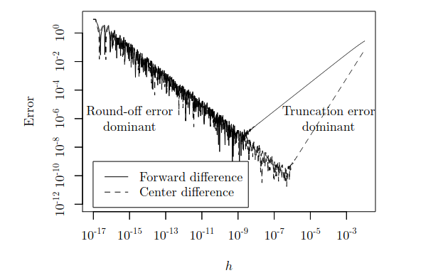
- Poor numerical stability
- Truncation Error: Finite Difference compute the slope of the secant line at $x$, rather than the tangent line at $x$
- Round-off Error: due to limited precision of the floating point operations, dividing a small number $h$ is inaccurate
- As $h \downarrow$, Truncation Error $\downarrow$, but Round-off Error $\uparrow$
- As $h \uparrow$, Round-off Error $\downarrow$, but Truncation Error $\uparrow$
- Implementation of Finite Difference has to consider the trade-off between Truncation Error and Round-off Error
- Computationally expensive
- Require $O(n)$ evaluation of $f$
- In deep learning, a model typically contains millions of parameters, rendering Finite Difference impractical
Symbolic Differentiation
Symbolic Differentiation produce analytical form of the derivative $f’$ for the target function $f$, following differentiation rules. It basically implement a software to compute the derivatives as human do. Symbolic Differentiation have 3 main problems:
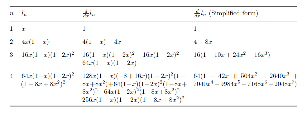
- Expression swell
- Some rules (e.g., product rule, quotient rule) produce 2 or more terms out of 1 expression. Without simplify the expression, total terms could grow at an exponential rate
- Requires closed form function
- This is a big problem for deep learning, as it is hard/expensive to express each parameter in a closed form function
- Computationally expensive
- Requires storing and computing $O(n)$ analytical expressions
- In deep learning, a model typically contains millions of parameters, rendering Symbolic Differentiation impractical
Consider a recursive expression: $l_{n+1} = 4 l_n(1 − l_n)$, where $l_1 = x$
Automatic Differentiation (AD)
Automatic Differentiation also compute derivative following differentiation rules. The key difference between AD and Symbolic Differentiation is: Symbolic Differentiation output expressions and use expressions to compute derivatives; AD computes derivatives directly. The key observation is that: All numerical computations are ultimately compositions of a finite set of elementary operations for which derivatives are known and combining the derivatives of the constituent operations through the chain rule gives the derivative of the overall composition. To illustrate this point, consider $f = \ln(x_1) + x_1x_2 − \sin(x_2)$. The computation graph is as follow:
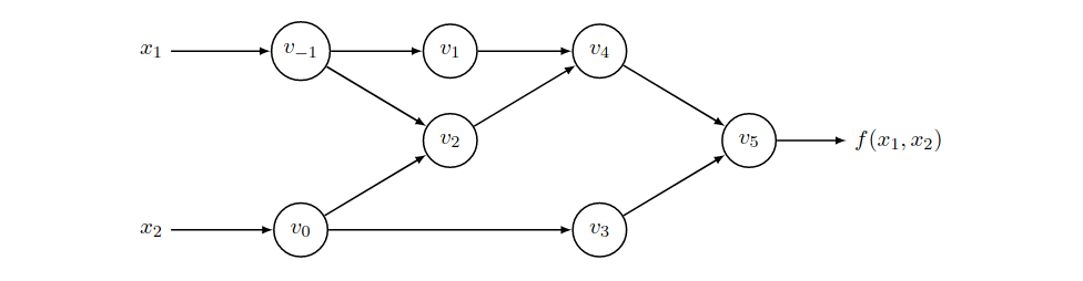
Function $f$ is decomposed into the above Computation Graph as follow:
- Node $v_{-1}, v_0$ takes input $x_1, x_2$
- Node $v_1 = \ln(x_1) = \ln(v_{-1})$
- Node $v_2 = x_1 x_2 = v_{-1} v_0$
- Node $v_3 = \sin(x_2) = \sin(v_0)$
- Node $v_4 = \ln(x_1) + x_1 x_2 = v_1 + v_2$
- Node $v_5 = \ln(x_1) + x_1 x_2 + \sin(x_2) = v_3 + v_4 $
Forward Mode
Forward mode propagates derivatives with respect to the independent variables in “forward” direction. $\dot{v_{-1}}$ represent taking derivative w.r.t some variable $x_i$. For example, when taking derivative w.r.t $x_1$, $\dot{v_{-1}} = \frac{\partial v_{-1}}{\partial x_1} = 1$ and $\dot{v_0} = \frac{\partial v_0}{\partial x_1} = 0$. $\dot{v_1}$ to $\dot{v_5}$ are obtained by following differentiation rules and chain rule. Below is a forward model evaluation trace:
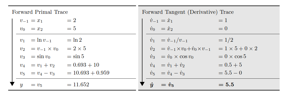
Consider a general mapping $f: \mathbb{R}^n \rightarrow \mathbb{R}^m$. Forward mode requires $O(n)$ evaluations to compute derivatives for all variables (setting $\dot{x_i} = 1$ and everything else to $0$). By setting $\dot{x}$ as an unit directional vector, forward model AD can compute directional derivative with $O(1)$ complexity.
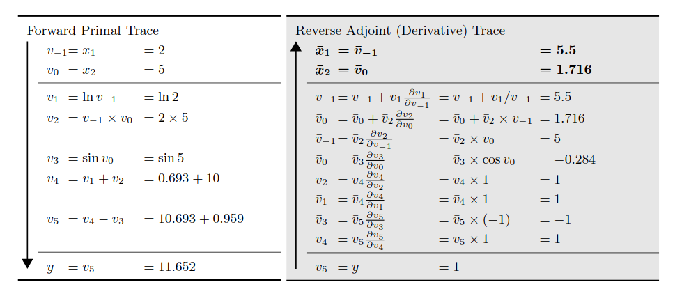
Reverse Mode
Reverse mode propagates derivatives with respect to the independent variables in “reverse” direction. $\bar{v_{-1}}$ represent taking derivative of $y$ w.r.t $v_i$. For example, $\bar{v_5} = \frac{\partial y}{\partial v_5} = 1$.
If we are interested in derivative w.r.t $x_1$, we will need $\bar{v_{-1}} = \frac{\partial y}{\partial v_{-1}}$. Looking at the computation graph, $v_{-1}$ can only affect $y$ through $v_1$ and $v_2$. Therefore,
\[\bar{v_{-1}} = \frac{\partial y}{\partial v_{-1}} = \frac{\partial y}{\partial v_1} \frac{\partial v_1}{\partial v_{-1}} + \frac{\partial y}{\partial v_2}\frac{\partial v_2}{\partial v_{-1}} = \bar{v_1} \frac{\partial v_1}{\partial v_{-1}} + \bar{v_2} \frac{\partial v_2}{\partial v_{-1}}\]Compute all $\bar{v_i}$ and we will have derivatives for all $x_i$ in one pass.
The efficiency of reverse mode come at the cost of increased storage requirements: in forward mode, you only need to maintain the nodes that associated with one $x_i$; in reverse mode, you need to maintain the nodes that associated with all $x_i$.
Forward Mode vs Reverse Mode
The key observation of AD is that chain rule is just a sequence of products and computing products in forward direction and reverse direction are equivalent.
- Forward Mode
- Computation initiated from $x_i$
- Each evaluation compute one column of the Jacobian matrix
- $\dot{v_k} = \frac{\partial v_k}{\partial x_j}$
- Reverse Mode
- Computation initiated from $y_j$
- Each evaluation compute one row of the Jacobian matrix
- $\bar{v_k} = \frac{\partial y_j}{\partial v_k}$
- Efficiency
- Consider a general mapping $f: \mathbb{R}^n \rightarrow \mathbb{R}^m$
- Forward mode computation cost $< n \cdot c \cdot \operatorname{ops}(f)$
- Reverse mode computation cost $< m \cdot c \cdot \operatorname{ops}(f)$
- $c=6$ and above are upper bounds for computation cost
- On average, you can achieve computation cost of $2 < c < 3$
Advantages of AD
- Compute derivatives without closed analytical expression
- Only requires operations in computation graph are differentiable
- Can handle branching, loops and recursion that are commonly used in scientific programming
- Highly efficient in deep leaning
- Since loss function has 1 output, reverse mode AD only requires O(1) complexity
- Comparing AD to Symbolic Differentiation or Finite Difference, the efficiency of AD compares from data reuse
- Both Symbolic Differentiation and AD relies on same differentiation rules. The key difference is Symbolic Differentiation walk through shared graph repeatedly for each $x_i$. Reverse mode AD stored the values on shared graph for each $x_i$.
- Finite Difference is even less efficient, it walk through full computation graph for each perturbation on $x$.