Automatic Differentiation Variational Inference
This post is mainly based on
Motivation
Recall in the Variational Inference post we discussed Coordinate Ascent Variational Inference (CAVI). We highlighted that CAVI cannot be generalized since each model requires a custom optimization / update rule. Once you make a small small change to the model, you need to hand derived everything. Another problem of CAVI’s analytical update is that it requires conjugacy. To add more color, you may interested in a Fireside Chat with David Blei where he talked about implementing the variational inference algorithm for Latent Dirichlet Allocation (LDA).
The motivation for Automatic Differentiation Variational Inference (ADVI), is to design a algorithm that can automatically derives an efficient variational inference algorithm. The authors posits that probabilistic programming is not the widely used due to designing the custom optimization algorithm is too hard. Researchers often have good domain knowledge over the generative process, but could not fit the probabilistic model. By automating the inference process, ADVI removes the main barrier for completing Bayesian Workflow.
ADVI
Rather than digging into details of the implementation, we will focus 4 high level problems ADVI need to solve:
- Latent variables transformation
- Compute gradient as Expectation
- Compute gradient over transformed latent variables
- Step-size selection for Stochastic gradient ascent
Latent variables transformation
Latent variables could have constraints. For example, the rate parameter for a poisson random variable must be positive. Without transformation, we will likely face a constrained optimization problem, which is harder to solve compared to unconstrained optimization problem. ADVI transform latent variable $\theta \in \mathcal{D}$ into $\zeta \in \mathbb{R}$ and solve unconstrained optimization problem for $\zeta$.
Compute gradient as Expectation
Recall in Variational Inference our key observation is that minimizing KL-divergence is equivalent to maximizing ELBO.
\[\mathcal{L}(q) = \mathbb{E}_{\theta \sim q(\theta)}\left[ \log \frac{p(\theta,D)}{q(\theta)} \right] = \mathbb{E}_{\theta \sim q(\theta)} [ \log p(\theta,D) - \log q(\theta) ]\]Here we know both $p(\theta,D)$ and $q(\theta)$. We also know how to take gradient with Automatic Differentiation (AD). The problem is we don’t know how to take gradient through the expectation of $\theta \sim q(\theta)$. The solution is compute gradient inside the expectation with AD and compute the expectation by Monte Carlo Integration. Recall that we can select $q(\theta)$ to be a simple distribution where we know how to efficiently sample from it.
Compute gradient over transformed latent variables
Since $\theta$ is transformed into $\zeta$, we have two mapping $\zeta = T(\theta)$ and $\theta = T^{-1}(\zeta)$. Write the joint distribution $p(\theta, x)$ in terms of $\zeta$,
\[p(\zeta, x) = p(T^{-1}(\zeta), x) | \det J_{T^{-1}}(\zeta) |\]Where $\det J_{T^{-1}}(\zeta)$ is the Jacobian of the inverse of $T$. This Jacobian term exists due to it accounts for how the transformation warps unit volumes and ensures that the transformed density integrates to one. Given the transformation, AD can take gradient on $T^{-1}$ and the determinant.
ADVI choose the transformed latent variable $\zeta$ to be Gaussian. As previously mentioned, it has two mode: Mean-field Gaussian and Full-rank Gaussian, where the former assumes latent variables are independent.
Step-size selection for Stochastic gradient ascent
Combining all previous steps, we know how to compute unbiased gradient through sampling and AD. ADVI choose to solve the optimization problem by Stochastic gradient ascent. The authors select steps size based on Robbins–Monro algorithm, which adds theoretical guarantee on convergence.
Experiments
Mean-field vs and Full-rank mode
The authors run ADVI on a Bivariate-Gaussian with $x_1$ and $x_2$ are correlated. The plot below show that mean-field mode can correctly identify the mean of the posterior, but underestimate the variance.
![]()
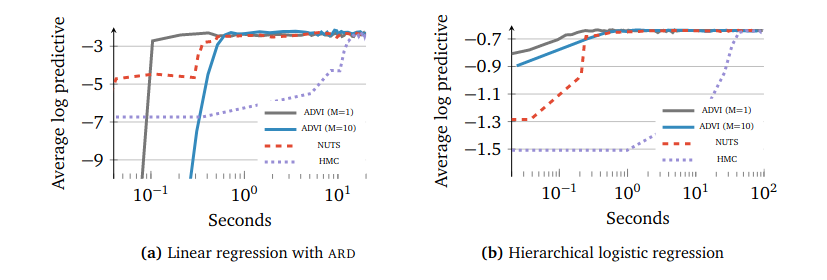
Speed of convergence
ADVI compute gradient by sampling from $z(\zeta)$, thus requires a hyperparameter of sample size $M$. One interesting finding is that take 1 sample is adequate for ADVI to converge.
Recall that we discussed the trade-off between MCMC and VI in Sampling from distribution post. The experiment below is a good example to show that VI can be significantly efficient that MCMC.