Sampling from distribution
You are given a non standard distribution $\operatorname{P}(x|\theta)$. How to sample from it? There are three class of method to sample from a arbitrary distribution: Rejection Sampling (RS), Markov chain Monte Carlo (MCMC) and Variational Inference (VI). I write this post as an overview of the above 3 class of algorithms; I will try to lay down intuitions and compare their differences.
Intuitions
- Rejection Sampling: throw darts to a enveloping region and only accept samples when the dart falling below the target distribution
- MCMC: generate samples by traversing a Markov chain which has the target distribution as its stationary distribution
- Variational Inference: use a “simple” distribution to approximate the target distribution and sample from the “simple” distribution
If the target distribution is low dimensional, rejection sampling can effectively generate samples. There is another parameter estimation technique called Importance Sampling (IS). Note that IS can be used to estimate summary statistic (e.g., mean) of a distribution; it cannot generate samples.
If the target distribution is high dimensional, MCMC or VI are better choices. Rejection Sampling will suffer from curse of dimensionality; the majorities of propsal will be rejected, resulting in low sampling efficiency.
The trade off between is more MCMC and VI are more subtle. MCMC is produced more “accurate” estimation, but are slow compared VI. By “accurate”, samples from MCMC are generated from the exact target distribution, but samples from VI is generated from the approximation distribution (but samples are still unbiased). In terms of when to choose MCMC or VI, David Blei’s review stated, VI is suitable for large data sets and scenarios where we want to quickly explore many models. MCMC is suited to smaller data sets and scenarios where we happily pay a heavier computational cost for more precise samples.
Rejection sampling
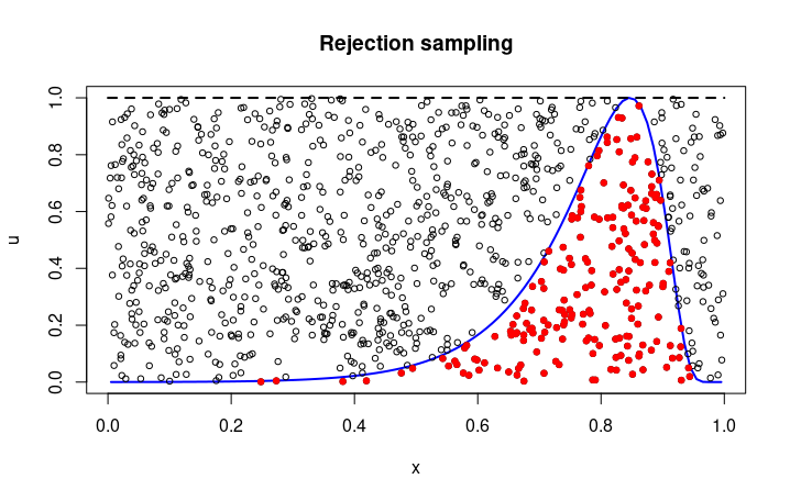
Rejection sampling is very easy to understand. As shown above, samples are generated by accepting red points (dart falling below the pdf of the target distribution).
Algorithm
Consider the target distribution $f(x)$, choose a proposal distribution g(x) and a real value $M$, where $Mf(x) \leq g(x), \forall x$
- Sample from proposal $x \sim g(x)$
- Accept the proposal with probability $\frac{f(x)}{Mg(x)}$
- Sample $u \sim \operatorname{Unif}(0,1)$
- If $u < \frac{f(x)}{Mg(x)}$, accept $x$, else reject $x$
Summary
- Support of $g(x)$ must covers support of $f(x)$
- Samples are generated independently
- Inefficient in high dimensional distributions or distributions with spikes
- Efficiency of RS is determined by the gap between $Mg(x)$ and $f(x)$
- In high dimensional space or distributions with spikes, $f(x) \ll Mg(x)$ for $x \sim g(x)$
- This result in high rejections rate and inefficient sampling
- However, RS could still be useful in practice, e.g., sampling the conditional distribution in Gibbs sampler
MCMC
Motivation
Recall that rejection sampling is inefficient when $f(x) \ll Mg(x)$ for most of $x \sim g(x)$. You can argue that this inefficiency originate from the design where each new sample is generated independently, ignoring all previous accepted samples. MCMC manages to overcome this inefficient by extracting information from the previous sample: it gains some knowledge about the distribution by looking at the previous sample, and pick the next sample based on this learned knowledge.
Stationary
MCMC aims generate samples by walking on the Markov chain which has the target distribution as stationary distribution. The question is how to design this Markov chain such that its stationary distribution is the target distribution. The design will be determined by specific MCMC algorithm. For example, the Metropolis-Hastings algorithm take an arbitrary Markov chain and adjusts it using the “accept-reject” mechanism to ensure the resulting Markov chain has the target distribution as its stationarity distribution.
Ergodic
MCMC algorithms construct Markov chain to have the target distribution as their stationary distribution. However, since we don’t know how to sample from stationary distribution and need to start from a random state, additional guarantee is required to ensure that the Markov chain will converge to the stationary distribution, i.e., the chain is ergodic. Formally, a Markov chain $\{X_n\}$ is ergodic if $\pi(j) = \lim_{n\to\infty} \operatorname{P}_i(X_n = j)$, where $\pi$ is stationary distribution, $n$ is step number, $j$ is any state and $i$ is the initial state.
Summary
- MCMC is a general framework which describe how samples could be generated; it does not describe a specific algorithm
- Samples are correlated
- There is a burn-in period, before the chain entered the stationary distribution
- Diagnostics are required (e.g., effective sample size, trace plot)
- Some popular MCMC algorithms
- Metropolis Hastings
- Gibbs Sampling
- Hamiltonian Monte Carlo (HMC)
- No-U-Turn Sampler (NUTS)
In practice, Metropolis Hastings is not very efficient due to rejection rate and autocorrelation. Gibbs Sampling is a special case of Metropolis Hastings which generate samples without rejections. Hamiltonian Monte Carlo (HMC) and No-U-Turn Sampler (NUTS) are developed to reduce autocorrelation. All of them will be discussed in future posts.
Variational Inference
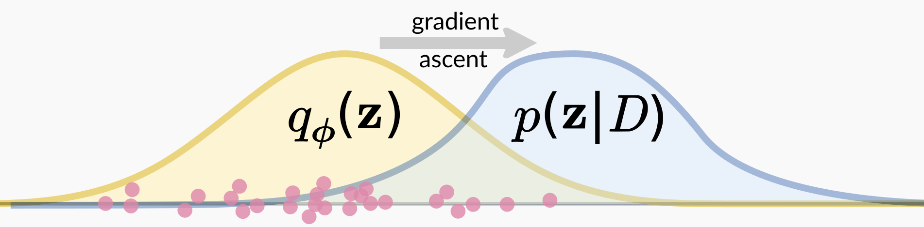 Visualization from blog of Matsen group
Rejection Sampling and MCMC generate samples directly from target distribution. Variational Inference take a different approach: it use a surrogate distribution to approximate the target distribution. The surrogate distribution is a simple distribution which you know how to sample from. And you generate samples from the surrogate distribution.
Consider the Bayesian inference problem where we try to estimate the posterior $\operatorname{P}(z|x=D)$. We choose a class of simple distribution $q(z)$ and optimize $q(z)$ to approximate $\operatorname{P}(z|x=D)$. Here $q(z)$ is a class of functions (say, all normal distributions), and it has is own parameters (say, mean $\mu$ and variance $\sigma^2$). To approximate $\operatorname{P}(z|x=D)$ with $q(z)$, we minimize their KL-Divergence.
Summary
- VI is a general framework which describe how samples could be generated; it does not describe a specific algorithm
- Samples are generated independently, but from the surrogate distribution
- The sampling problem is turned into an optimization problem: $\operatorname{argmin}_{q \in \mathcal{Q}} \operatorname{KL}(q(z) || \operatorname{P}(z|x=D))$
- Diagnostics are required (e.g., ELBO plot)
- Some popular MCMC algorithms
- Mean Field Approach
- Coordinate Ascent Variational Inference (CAVI)
- Automatic Differentiation Variational Inference (ADVI)
Mean Field Approach describes a possible assumption of surrogate distribution: each $z_i$ is independent of others. CAVI is an implementation of MFVI and requires manual derivation of update rule for each $z_i$ (generally faster that ADVI since you have an analytical solution for each coordinate). ADVI requires no derivation and uses automatic differentiation to directly optimization $q(z)$. You can choose to implement ADVI using Mean-field approach. You can also drop the independent $z_i$ assumption: suppose the surrogate distribution is normal, dropping the independent $z_i$ assumption means you need to optimize a full-rank covariance matrix to describe the correlation between axis.