S4: Structured State Space Models
This post is mainly based on
- Efficiently Modeling Long Sequences with Structured State Spaces, ICLR 2022
- Seminar - Albert Gu | Stanford MLSys #46
- Why S4 is Good at Long Sequence: Remembering a Sequence with Online Function Approximation
- The Annotated S4
There are 3 paradigms for modelling long time series: Continuous-Time Model (CTM), RNN and CNN
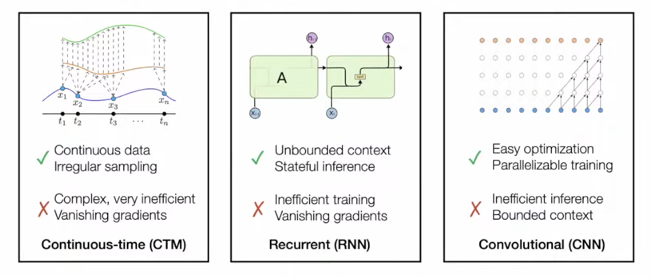
Existing architectures cannot handle extremely long sequence (10000+ steps), due to:
- CTM: hard to optimize
- CNN: receptive field is fix; high inference memory; large receptive field requires large filter / deep architecture
- RNN: forgetting problem
- Transformer: $O(n^2)$ memory complexity for attention matrix
The Structured State Space Model (S4) unify CTM, CNN and RNN.
- S4 has 3 different types of representations, corresponding to CTM, CNN and RNN
- S4 can switch between the 3 representations
Background
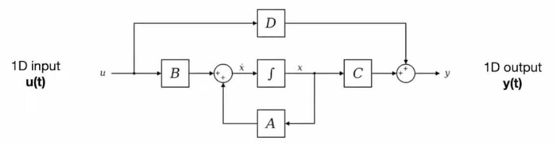
Linear State Space Model (Linear SSM)
\[\begin{align} x'(t) &= Ax(t) + Bu(t) \\ y(t) &= Cx(t) + Du(t) \end{align}\]where,
- Input $u \in \mathbb{R}$
- State $x \in \mathbb{R}^N$
- $ A \in \mathbb{R}^{N \times N}, B \in \mathbb{R}^{N \times 1}, C \in \mathbb{R}^{1 \times N}, D\in \mathbb{R}^{1 \times 1} $
The above form is known as continuous time representation of SSM
For detail on linear SSM, please refer to discussions on Linear State Space Layer.
HiPPO
- A class of matrices $A \in \mathbb{R}^{N \times N}$
- $A$ allows the state $x(t)$ to memorize the history of input $u(t)$
- LSSL adopt such matrix $A$ and outperform various SOTA model on long range time series benchmarks
3 Representations of SSM
The SSM has 3 different types of representations: Continuous-time, Recurrent and Convolutional.
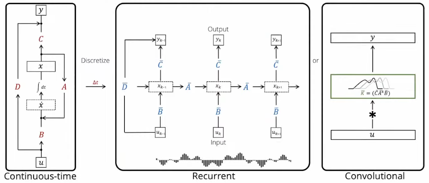
Continuous-Time Representation
The continuous-time representation correspond to the function to function map: $u(t) \rightarrow y(t)$, which cannot be directly estimated from the discrete data $(u_0, y_0), …, (u_k, y_k)$.
Recurrent Representation
A continuous SSM($A,B,C,D$) can be discretize into SSM($\bar{A},\bar{B},\bar{C},\bar{D}$), where
The above transformation between continuous and discrete form is well studied. Refer to discussions around Generalized Bilinear Transform (GBT).
To simplify the discussion, assume $D = 0$. The reason is $D$ can be viewed as a skip connection of input $u$ and is easy to estimate.
Let the step size between $u_t$ and $u_{t-1}$ be $\Delta$, then we have the discrete SSM:
\[\begin{align} \bar{A} &= (I - \Delta/2 \cdot A)^{-1}(I + \Delta/2 · A) \\ \bar{B} &= (I - \Delta/2 \cdot A)^{-1} \Delta B \\ \bar{C} &= C \end{align}\]The Recurrent Representation of the SSM can be viewed as an RNN, as discussed in the Expressivity of LSSL.
Convolutional Representation
The recurrent representation can be unrolled into convolutional form: for $i \leq j$, each input $u_i$ is passed through $\bar{B},\bar{C}$ matrices 1 time and $\bar{A}$ matrix $j-i$ times
The above computation is equivalent to a CNN with a $L$-length 1D convolutional filter $\bar{K}$:
\[\bar{K} \in R^L := (\bar{B}\bar{C}, \bar{C}\bar{A}\bar{B}, ..., \bar{C}\bar{A}^{L-1}\bar{B})\] \[y = \bar{K} * u\]Advantage of Each Representation
- Continuous-Time: theoretical grounded and easy to analyze (e.g., long term memory, sampling resolution change)
- Recurrent: constant memory requirement in autoregressive sequence generation
- Convolutional: parallel training
Technical Challenges of SSM
Problem 1: $A$ need to be carefully initialized to enable SSM to learn long-range dependencies
As discussed in LSSL post, if $A$ is randomly initialized, SSM performs poorly in very simple sequence modelling task.
If $A$ is initialized as a HiPPO Matrix:
\[A_{nk} = \begin{cases} (2n+1)^{\frac{1}{2}}(2k+1)^{\frac{1}{2}} & \text{if } n>k \\ n+1 & \text{if } n=k \\ 0 & \text{if } n<k \end{cases}\] \[B_n = (2n+1)^{\frac{1}{2}}\]The state sequence $x_0, …, x_k$ will try to memorize $u_0, …, u_k$.
Refer to HiPPO & Sequential Data Compression post.
On sequential MNIST problem,
- $A \sim \mathcal{N}(0,1)$: 60% accuracy
- $A \sim \operatorname{HiPPO}$: 98% accuracy
Problem 2: direct computation of the convolution kernel $\bar{K}$ is costly and numerically unstable
- Computing $\bar{K}$ involves repeated matrix multiplication $\bar{A}^{L-1}$
- This could be unstable if $\bar{A}$ has the largest eigenvalue not close to 1.
- Automatic differentiation through $\bar{A}^{L-1}$ also leads to vanishing gradient problem
- Computing $\bar{A}^{L-1}$ leads to $O(N^2L)$ complexity. Ideally, we want $O(L)$ complexity
Structured SSM (S4)
The LSSL paper attempted to address the Problem 2, however, the proposed method is unsuccessful:
- Theorem 2 is proposed to efficiently compute convoluational kernel $\bar{K}$
- However, the authors found that the algorithm implied by Theorem 2 is numerically unstable
- For details, see discussions on Limitations of LSSL.
S4 proposed a new parameterization on how to efficiently compute kernel $\bar{K}$.
The authors discussed:
- Conjugation and Diagonalization of $A$
- Normal Plus Low-Rank Decomposition improves naive Diagonalization
- Discussions on computation and space complexity
Conjugation / Diagonalization of HiPPO Matrix $A$
The problem with the CNN kernel $ \bar{K} := (\bar{B}\bar{C}, \bar{C}\bar{A}\bar{B}, …, \bar{C}\bar{A}^{L-1}\bar{B}) $, is the repeated matrix multiplication by $\bar{A}$.
The first attempt is to solve this by Conjugation.
Diagonalization
\[A=VDV^{-1}\]where,
- $D$ is diagonal
- $V$ is composed of the eigenvectors of $A$
Jordan Canonical Form
\[A=VJV^{-1}\]where,
- $J$ is block diagonal
- $V$ is composed of the generalized eigenvectors of $A$
Generalized Eigenvectors
- A generalized eigenvector of order $k$ is a nonzero vector $v$ that satisfies
- $(A-\lambda I)^kv=0$ for some eigenvalue $\lambda$
- $(A-\lambda I)^{k-1}v \not=0$
- The case where $k=1$ corresponds to regular eigenvectors
- Why Generalized Eigenvectors?
- Generalized eigenvectors is useful when $A$ does not have enough linearly independent eigenvectors to diagonalize it
- This is often due to some eigenvalues having a higher algebraic multiplicity than geometric multiplicity
- The generalized eigenvectors form what is known as the generalized eigenspace for the eigenvalue $\lambda$. They provide a basis for the Jordan blocks in the Jordan canonical form of $A$.
- Jordan Canonical Form
- Each Jordan block corresponds to an eigenvalue and is associated with a chain of generalized eigenvectors
- The first vector in the chain is a regular eigenvector (generalized eigenvector of order 1)
- The subsequent vectors in the chain are higher-order generalized eigenvectors
Conjugation
Let
- $A$ be a square matrix
- $V$ be an invertible matrix
The conjugate of $A$ by $V$, denoted $A’$, is defined as the matrix
\[A'=V^{-1}AV\]where,
- $A’$ is not necessary diagonal / block diagonal
- $V$ is not necessarily composed of the eigenvectors of $A$
This process maps $A$ to a new matrix $A’$ using $V$:
- $V^{-1}$ transforms the coordinate system, moving from the standard basis to the new basis defined by $V$
- $A$ is then applied in this new basis, performing the transformation that $A$ represents
- Finally, $V$ transforms the coordinate system back to the original basis
Properties
- Conjugation is a change of basis operation in linear algebra that doesn’t alter the linear transformation’s action on the space
- Hence, conjugation maintains the eigenvalues of $A$ and, more generally, its spectral properties
Relationships
- Jordan Canonical Form is a special case of Conjugation
- Diagonalization is a special case of Jordan Canonical Form
Lemma 3.1
Conjugation is an equivalence relation on SSMs $(A,B,C) \sim (V^{-1}AV, V^{-1}B, CV)$.
SSM$(A,B,C)$:
\[\begin{align} x'(t) &= Ax(t) + Bu(t) \\ y(t) &= Cx(t) \end{align}\]SSM$(V^{-1}AV, V^{-1}B, CV)$:
\[\begin{align} \tilde{x}'(t) &= V^{-1}AV \tilde{x}(t) + V^{-1}Bu(t) \\ y(t) &= CV \tilde{x}(t) \end{align}\]The above 2 systems are equivalent. You can verify this by substituting $ x(t) = V\tilde{x}(t) $ (change of basis of state $x$) for SSM$(A,B,C$), you will get SSM$(V^{-1}AV, V^{-1}B, CV)$.
Unfortunately, the naive application of diagonalization does not work due to numerical stability issues.
Normal Plus Low-Rank (NPLR) Decomposition
The numerical stability issues emerged from the discussion above implies that we should only conjugate by well-conditioned matrices $V$.
- The ideal scenario is $A$ is diagonalizable by a perfectly conditioned matrix
- i.e., unitary matrix / absolute value of eigenvalue = 1 / norm-preserving
- By the Spectral Theorem of linear algebra, this requires $A$ to be normal matrices
- However, HiPPO matrix is not normal matrix
However, HiPPO matrix can be decomposed as the sum of a normal matrix and a low-rank matrix.
This decomposed is still not useful by itself:
- Unlike a diagonal matrix, powering up this sum of 2 matrices is still slow and not easily optimized
- 3 techniques are required to make it useful
- Truncated generating function
- Woodbury identity
- Cauchy kernel
We will skip details on NPLR since the author later discovered that the “easy to implement” diagonal state space model (S4D) is equally effective as S4.
Theorem 1
All HiPPO matrices have a Normal Plus Low-Rank (NPLR) representation:
\[A = V \Lambda V^∗ − P Q^\top = V (\Lambda - ( V^* P ) (V^* Q)^*) V^*\]where
- $V \in \mathbb{C}^{N \times N}$ is unitary
- $\Lambda$ is diagonal
- $P, Q \in \mathbb{R}^{N \times r}$ is low-rank factorization
S4 Computational Complexity
Theorem 2 (S4 Recurrence)
Given any step size $\Delta$, computing one step of the SSM recurrence can be done in $O(N)$ operations where $N$ is the state size
Theorem 3 (S4 Convolution / S4’s core technical contribution)
Given any step size $\Delta$, computing the SSM convolution filter $\bar{K}$ can be reduced to 4 Cauchy multiplies, requiring only $O(N + L)$ operations and $O(N + L)$ space
S4 Layer Architecture
Following the NPLR Decomposition, an S4 layer is parameterized as a SSM $ (\Lambda - PQ^*, B, C) $, which contains 5 trainable parameters.
Follow-up work found that this version of S4 can sometimes suffer from numerical instabilities when the A matrix has eigenvalues on the right half-plane. It introduced a slight change to the NPLR parameterization for S4 from $ \Lambda - PQ^* $ to $ \Lambda - P P^* $ that corrects this potential problem.
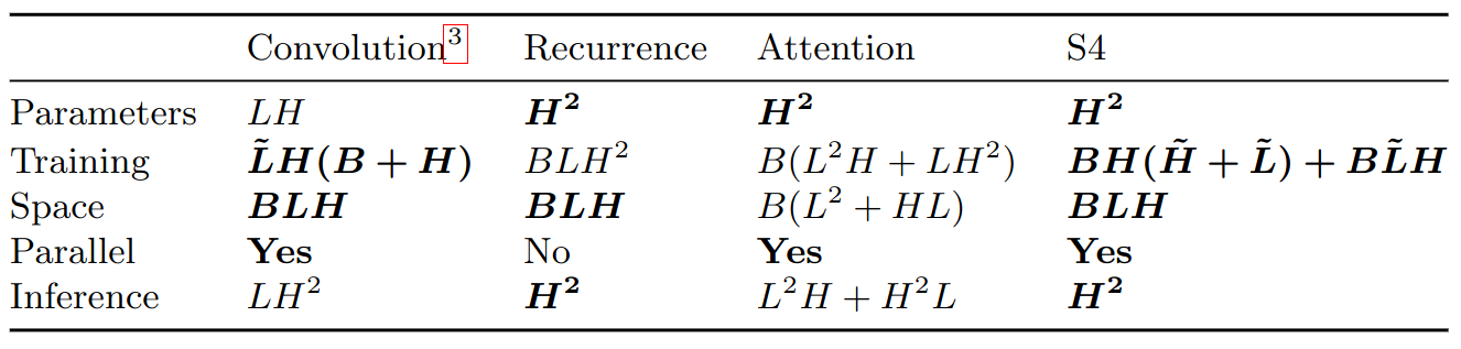
Complexity of various sequence models in terms of sequence length (L), batch size (B), and hidden dimension (H).
Experiments
Efficiency Benchmarks
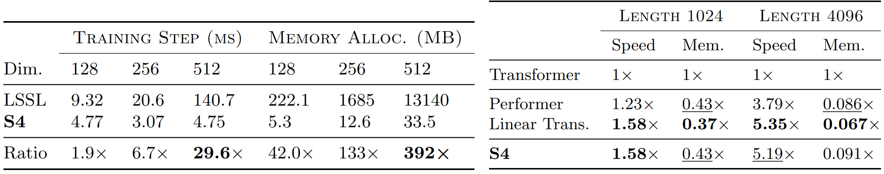
Left: The S4 parameterization with NPLR is asymptotically more efficient than the LSSL.
Right: S4 vs efficient Transformers. S4’s speed and memory use is competitive with the most efficient Transformer in a parameter-matched setting.
Long Range Dependency (LRD) Benchmarks
Long Range Arena (LRA)
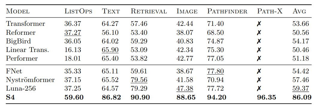
Performance on Long Range Arena. Tasks are extremely challenging (e.g., Path-X requires reasoning about LRDs over sequences of length $128 \times 128 = 16384$). S4 significantly outperforms SOTA models. For reproducibility, read paper’s Appendix D.5.
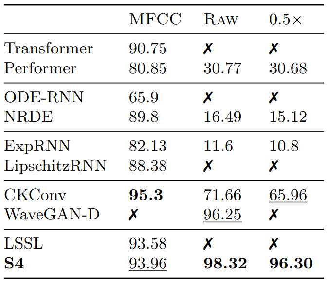
Speech Classification
- SC10 subset of the Speech Commands dataset (length-16000)
- S4 achieves 98.3% accuracy, higher than all baselines that use the 100x shorter MFCC features
- S4 outperforms WaveGAN-D, a CNN specifically designed for raw speech. WaveGAN-D has 90x more parameters and incorporating many architectural heuristics
General Sequence Model
Experiments are to test model performance on general sequential data, including
- Discriminative modelling on
- Flattened image
- Randomly permuted image (permutation is fixed)
- Generative modelling on
- Image
- Text
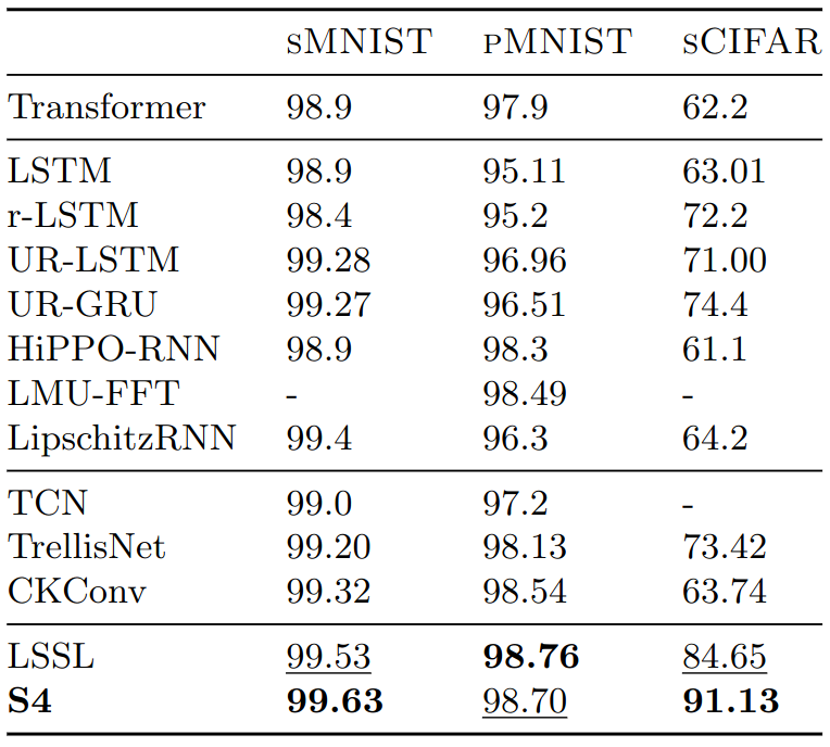
Discriminative modelling / Pixel-level 1-D image classification
Generative modelling / CIFAR-10 density estimation
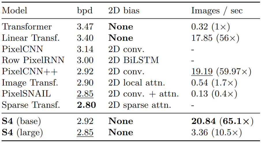
CIFAR image are $32 \times 32$ pixel images with 3 color channels. Each image consists of $32 \times 32 \times 3 = 3072$ RGB values.
To compute bits per dim, each image is flattened and an auto-regressive model can predicted conditional probability for each of the 3072 steps:
\[p_1, p_2, ...., p_{3072}\]Then we can compute the total log likelihood:
\[\text{Total Log Likelihood} = \sum_{i=1}^{3072} \log (p_i)\]A higher total log likelihood indicates that the model is doing a better job of predicting each subpixel, meaning it has learned a more accurate representation of the data distribution.
The total log likelihood is then normalized and convert to base 2:
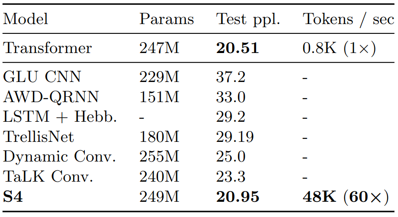
\[\text{Bits per Dimension} = \frac{ \text{Total Log Likelihood} }{ 3072 \cdot \log(2)}\]Generative modelling / WikiText-103 language modeling
Ablations
To answer the question:
- How important is the HiPPO initialization?
- How important is training the SSM on top of HiPPO?
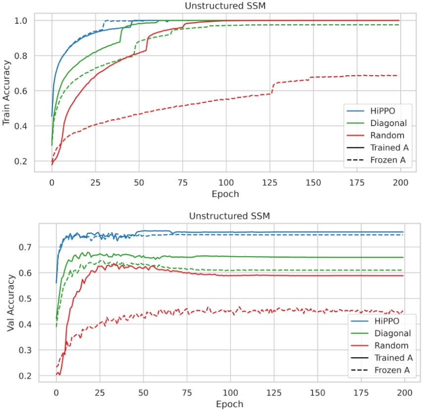
CIFAR-10 classification with unconstrained, real-valued SSMs with various initializations. Top: Train accuracy. Bottom: Validation accuracy. For all methods, training the SSM led to improvements in both training and validation curves. However, different initialization results in largely different generalization gaps.