HiPPO & Sequential Data Compression
This post is mainly based on
HiPPO? Hippocampus? Memory!
- HiPPO = High-order Polynomial Projection Operators
- Online compression of time series by projection onto polynomial bases
- Online: representing history in an incremental fashion as more data is processed
- Compression: given a measure that specifies the importance of each time step in the past, produces an optimal solution to the approximation problem
- HiPPO-LegS
- A new memory update mechanism
- Advantage
- Timescale / sampling rates robustness
- Fast updates
- Bounded gradients
- Results
- New SOTA on pMNIST, outperforming all RNN and transformer based models
- Trajectory classification: outperforming RNN and neural ODE by 25-40%
Memory = Online Function Approximation
Given a time series function $f(t)$:
\[f(t): \mathbb{R}_+ \rightarrow \mathbb{R}\]$f(t)$ takes non-negative real valued time $t$ and map it to any real value.
Consider memorizing $f(t)$ by mapping it to a set of optimal coefficients w.r.t some basis functions. The approximation is evaluated with respect to a measure that specifies the importance of each time in the past.
The basis functions: orthogonal polynomials (OPs).
Why choosing orthogonal polynomials (OPs) as basis functions?
- The optimal coefficients of OPs can be expressed in closed form
- OPs are well-studied
- OPs are widely use in approximation theory and signal processing
HiPPO is developed as a framework, which can produces operators that project arbitrary functions onto the space of orthogonal polynomials with respect to a given measure. The paper presented 3 different measures:
- HiPPO-LegT: Translated Legendre, equal weight on $[t-\theta, t]$
- HiPPO-LagT: Translated Laguerre, exponential decaying weight on $[t-\theta, t]$
- HiPPO-LegS: Scaled Legendre, equal weight on $[0, t]$
HiPPO can be viewed as a closed-form ODE or linear recurrence, allows fast incremental updating of the optimal polynomial approximation as the input function is revealed through time.
HiPPO framework is a generalization many past works
- LMU: special case of HiPPO-LegT
- Gated RNN: special case of HiPPO-LagT
HiPPO is closely connected to dynamical systems and approximation theory. This allow us to show several theoretical benefits of HiPPO-LegS:
- Invariance to input timescale
- Asymptotically more efficient updates
- Bounds on gradient flow and approximation error
The HiPPO Framework
Problem Setup
Given a time series function $f(t) \in \mathbb{R}$ where $t \geq 0$, many problems require operating on the cumulative history
\[f_{\leq t} := f(x) | x \leq t\]At every time $t \geq 0$, in order to understand the inputs seen so far and make future predictions.
To create and maintain (online) the compressed representation of the history $ f_{\leq t} $, we project $ f_{\leq t} $ onto a subspace of bounded dimension.
Two ingredients are required to fully specify this problem:
- A way to quantify the approximation (a measure / distance in function space)
- A suitable subspace
Function Approximation with respect to a Measure
Any probability measure $\mu$ on $[ 0, \infty )$ equips the space of square integrable functions with inner product
\[\langle f, g \rangle_\mu = \int_{0}^{\infty} f(x) g(x) \, d\mu(x)\]Polynomial Basis Expansion
Any N-dimensional subspace $\mathcal{G}$ of this function space $ f_{\leq t} $ is a suitable candidate for the approximation. The parameter $N$ corresponds to the order of the approximation.
Online Approximation
Since we need to approximate $ f_{\leq t} $ for every time $t$, the measure also need to vary through time.
For every $t$, $\mu^{(t)}$ is a measure supported on $(-\infty, t]$.
We seek some $g^{(t)} \in \mathcal{G}$ that minimize
\[\| f_{\leq t} - g^{(t)} \|_{L_2(\mu^{(t)})}\]where,
- $\mu^{(t)}$ is a weighted error measure
- $\mathcal{G}$ defines the allowable approximations
Challenges are
- How to solve the optimization problem in closed form given $\mu^{(t)}$
- How to maintained these coefficients online as $t \rightarrow \infty$
General HiPPO Framework
The HiPPO framework provides a simple and general solution for many measure families $\mu(t)$.
Why choosing measure $\mu(t)$ is important?
- Different time series modeling problems could have different history dependency
- For example, some problem could have strong long-term history dependency, while others don’t
- The user can choose appropriate $\mu(t)$ to reflect dependency
- The user’s choice of measure will lead to solutions with qualitatively different behavior
For more details, see Appendix A.1 and C.
Mapping f(t) to Coefficients of Orthogonal Polynomials
The classic approximation theory tells us:
If a set of basis functions ${g_n}$ forms an orthogonal basis in a function space, then any function $f$ within that space or its subspace can be approximated as a linear combination of these basis functions.
The coefficients $c^{(t)}_n$ of this linear combination in the optimal basis expansion are determined by the inner product (or projection) of the function $f$ onto each basis function $g_n$:
\[c^{(t)}_n := \langle f_{\leq t}, g_n \rangle_{ \mu^{(t)}}\]where,
- \(\langle \cdot, \cdot \rangle_{ \mu^{(t)}}\) the inner product with respect to a measure $\mu^{(t)}$
- $g_n$ is the nth basis function in the orthogonal basis
This principle is a cornerstone in various fields such as signal processing and functional analysis, enabling efficient representation and approximation of functions.
The HiPPO Abstraction
Definition 1. Given:
- A time-varying measure family $\mu^{(t)}$ supported on $(- \infty, t]$
- An $N$-dimensional subspace $\mathcal{G}$ of polynomials
- A continuous function $f: \mathbb{R}_{\geq 0} \to \mathbb{R}$
HiPPO, at every time $t$, defines:
- A projection operator $\text{proj}_t$
- A coefficient extraction operator $\text{coef}_t$
with the following properties:
$\text{proj}_t$ maps \(f_{\leq t}\) to a polynomial $g^{(t)} \in \mathcal{G}$ (the subspace spanned by polynomial basis), that minimizes the approximation error \(\|f_{\leq t} - g^{(t)}\|_{L_2(\mu^{(t)})}\)
$\text{coef}_t: \mathcal{G} \to \mathbb{R}^N$ maps the polynomial $g^{(t)}$ to the coefficients $c(t) \in \mathbb{R}^N$ of the basis of orthogonal polynomials defined with respect to the measure $\mu^{(t)}$
The composition $\text{coef} \circ \text{proj}$ is called hippo, which is an operator mapping a function \(f: \mathbb{R}_{\geq 0} \to \mathbb{R}\) to the optimal projection coefficients $c : \mathbb{R}_{\geq 0} \to \mathbb{R}^N$:
\[\left[ \text{hippo}(f) \right](t) = \text{coef}_t(\text{proj}_t(f))\]For each $t$, the problem of optimal projection $\text{proj}_t(f)$ is well-defined by the above inner products, but this is intractable to compute naively.
In Appendix D, the authors show that the coefficient function $ c(t) = \text{coef}_t(\text{proj}_t(f)) $ has the form of an ODE satisfying
\[\frac{d}{dt}c(t) = A(t)c(t) + B(t)f(t)\]for some $ A(t) \in \mathbb{R}^{N \times N}, B(t) \in \mathbb{R}^{N \times 1} $
This implies that $c(t)$ can be obtained online by solving an ODE, or more concretely by running a discrete recurrence. When discretized, HiPPO takes in a sequence of real values and produces a sequence of $N$-dimensional vectors.
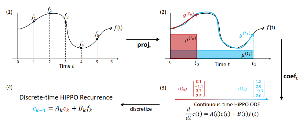
Illustration of the HiPPO framework. (1) For any function $f$, (2) at every time $t$ there is an optimal projection $g^{(t)}$ of $f$ onto the space of polynomials, with respect to a measure $μ^{(t)}$ weighing the past. (3) For an appropriately chosen basis, the corresponding coefficients $c(t) \in \mathbb{R}^N$ representing a compression of the history of $f$ satisfy linear dynamics. (4) Discretizing the dynamics yields an efficient closed-form recurrence for online compression of time series $f_k$ where $k \in \mathbb{N}$.
Measure Families and HiPPO ODEs
The main theoretical results are instantiations of HiPPO for various measure families, including 2 sliding window measures (LegT, LagT) and 1 scaled measure (LegS, measure on entire history). The authors also showed that the scaled measure has several advantages, which will be discussed later.
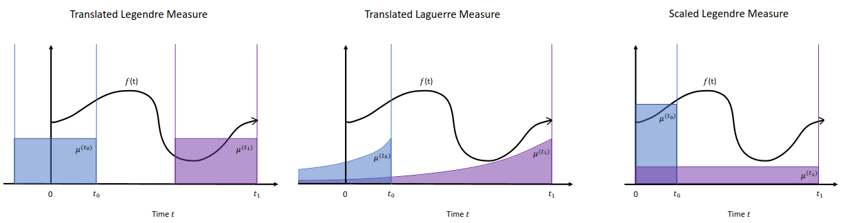
Illustration of different HiPPO measures at $t_0$ (blue) and $t_1$ (purple). Left: LegT measure. Middle: LagT measure. Right: LegS measure.
The unified perspective on memory mechanisms allows the authors to derive these closed-form solutions with the same strategy, provided in Appendices D.1, D.2.
Translated Legendre (LegT) measure assigns uniform weight to the most recent history $[t - \theta, t]$. There is a hyperparameter $\theta$ representing the length of the sliding window, or the length of history that is being summarized.
\[\text{LegT}: \mu^{(t)}(x) = \frac{1}{\theta} \mathbb{I}_{[t-\theta,t]}(x)\]Translated Laguerre (LagT) measure adopts exponentially decaying weight, assigning more importance to recent history.
\[\text{LagT}: \mu^{(t)}(x) = e^{-(t-x)} \mathbb{I}_{(-\infty,t]}(x) = \begin{cases} e^{x-t} & \text{if } x \leq t \\ 0 & \text{if } x > t \end{cases}\]Theorem 1. For $\text{LegT}$ and $\text{LagT}$ measure, the hippo operators satisfying Definition 1 are given by linear time-invariant (LTI) ODEs
\[\frac{d}{dt}c(t) = -Ac(t) + Bf(t)\]where $ A \in \mathbb{R}^{N \times N}, B \in \mathbb{R}^{N \times 1} $:
For LegT:
\[A_{nk} = \frac{1}{\theta} \begin{cases} (-1)^{n-k} (2n + 1) & \text{if } n \geq k, \\ 2n + 1 & \text{if } n \leq k, \end{cases} \quad B_n = \frac{1}{\theta} (2n + 1)(-1)^n\]For LagT:
\[A_{nk} = \begin{cases} 1 & \text{if } n \geq k, \\ 0 & \text{if } n < k, \end{cases} \quad B_n = 1\]LegT measure’s update equation and $A,B$ aligned with LMU’s update update equation.
ODE Discretization & HiPPO recurrences
Since actual data is inherently discrete (e.g. sequences and time series), the authors discuss how the HiPPO projection operators can be discretized using standard techniques, so that the continuous-time HiPPO ODEs become discrete-time linear recurrences.
Euler Method for ODE Discretization
Consider the derivative as a function of $t, c(t), f(t)$:
\[\frac{d}{dt} c(t) = u(t, c(t), f(t))\]Choose a step size $\Delta t$ and performs the discrete updates:
\[c(t + \Delta t) = c(t) + \Delta t \cdot u(t, c(t), f(t))\]Note that Euler Method is sensitive to choice of $\Delta t$ and is for or illustration purpose only. The authors conduct experiments with numerically stable Bilinear and ZOH methods. See Appendix B.3 for details.
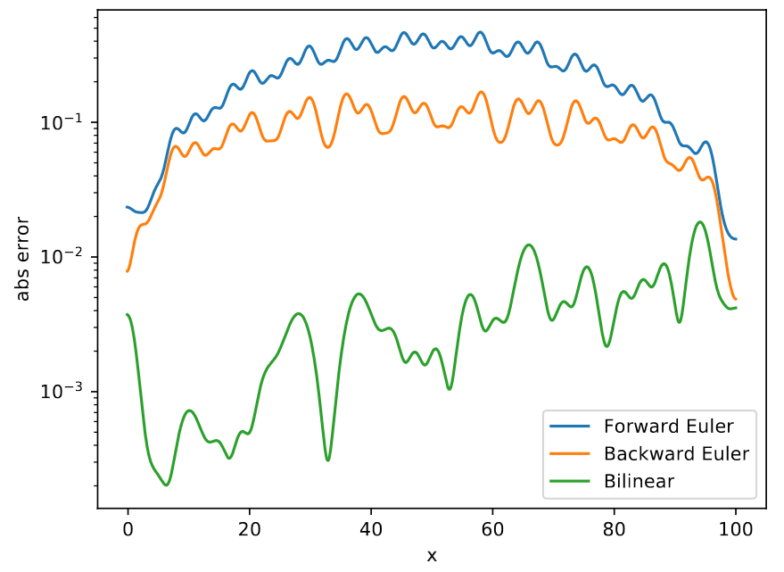
Absolute error for different discretization methods. Forward and backward Euler are generally not very accurate, while bilinear yields more accurate approximation.
Relationship to Gated RNNs
Consider Low Order Projection where number of basis $N=1$, then the iscretized version of HiPPO-LagT becomes:
\[\begin{aligned} c(t + \Delta t) &= c(t) + \Delta t(-Ac(t) + B f(t)) \\ &= (1 − \Delta t)c(t) + \Delta t f(t) \end{aligned}\]Consider $\Delta t$ be a function $f$ which takes $f(t), c(t)$ as input and out put a real number, then the above equation becomes a Gated RNNs. Compare the above update equation to GRU hidden state $h_t$’s update function.
The key differences are:
- HiPPO: uses one hidden feature, but projects it onto high order polynomials
- Gated RNNs: use many hidden features, but only project them with degree 1
HiPPO-LegS
Although sliding windows are common in signal processing, a more intuitive approach for memory should scale the window over time to avoid forgetting.
The scaled Legendre measure (LegS) assigns uniform weight to all history $[0, t]: \mu^{(t)} = \frac{1}{t}\mathbb{I}_{[0,t]}$
Theorem 2
The continuous time dynamics for HiPPO-LegS are:
\[\frac{d}{dt} c(t) = -\frac{1}{t} Ac(t) + \frac{1}{t} Bf(t)\]The discrete time dynamics for HiPPO-LegS are:
\[c_{k+1} = \left( 1 - \frac{A}{k} \right) c_k + \frac{1}{k} Bf_k\]where,
\[A_{nk} = \begin{cases} (2n+1)^{\frac{1}{2}}(2k+1)^{\frac{1}{2}} & \text{if } n>k \\ n+1 & \text{if } n=k \\ 0 & \text{if } n<k \end{cases}\] \[B_n = (2n+1)^{\frac{1}{2}}\]Timescale Robustness
The HiPPO-LegS operator is timescale-equivariant: dilating the input $f$ does not change the approximation coefficients.
Proposition 3
For any scalar $\alpha > 0$, if $h(t) = f(\alpha t)$, then
\[\text{hippo}(h)(t) = \text{hippo}(f)(\alpha t)\]In other words, if $\gamma : t \to \alpha t$ is any dilation function, then
\[\text{hippo}(f \circ γ) = \text{hippo}(f ) \circ \gamma\]The discrete recurrence is invariant to the discretization step size. The reason is that HiPPO-LegS have a linear ODE of the form:
\[\frac{d}{dt}c(t) = \frac{1}{t}Ac(t) + \frac{1}{t}Bf(t)\]which is different from LegT and LagT’s ODE: $\frac{d}{dt}c(t) = -Ac(t) + Bf(t)$
Apply GBT discretization to HiPPO-LegS’s linear ODE, we obtain:
\[c(t + \Delta t) = \left( I - \frac{\Delta t}{t + \Delta t}\alpha A \right)^{-1}\left( I + \frac{\Delta t}{t}(1 - \alpha)A \right)c(t) + \frac{\Delta t}{t}(I - \frac{\Delta t}{t + \Delta t}\alpha A)^{-1}Bf(t)\]This system is invariant to the discretization step size $\Delta t$.
Let $c^{(k)} := c(k\Delta t)$ and $f_k := f(k\Delta t)$, then we have the recurrence:
\[c^{(k+1)} = \left( I - \frac{1}{k + 1}\alpha A \right)^{-1}\left( I + \frac{1}{k}(1 - \alpha)A \right)c^{(k)} + \frac{1}{k}(I - \frac{1}{k + 1}\alpha A)^{-1}Bf_k\]which does not depend on the discretization step size $\Delta t$. (paper Appendix B.3)
Computational Efficiency
Note that a general discretization requires $O(N^2)$ operations. However, the LegS operators use a fixed $A$ matrix with special structure that turns out to have fast multiplication.
Proposition 4
Under any generalized bilinear transform discretization above, each step of the HiPPO-LegS recurrence $c_k \to c_{k+1}$ can be computed in $O(N)$ operations.
Gradient flow
LegS avoids the vanishing gradient issue.
Proposition 5
For any times $t_0 < t_1$, the gradient norm of HiPPO-LegS operator for the output at time $t_1$ with respect to input at time $t_0$ is
\[\left\| \frac{\partial c(t_1)}{\partial f (t_0)} \right\| = \Theta (1/t_1)\]Approximation error bounds
The error rate of LegS decreases with the smoothness of the input.
If a function $f$ has order-k bounded derivatives, then $f$ is k-times differentiable and that all derivatives up to the $k$-th order are bounded by some constant $M$ over the domain of $f$:
\[∣f^{(k)}(x)∣ \leq M\]Proposition 6
Let $f: R^+ \to R$ be a differentiable function, and let $g(t) = \text{proj}_t(f)$ be its projection at time $t$ by HiPPO-LegS with maximum polynomial degree $N − 1$. If $f$ is L-Lipschitz then,
\[\| f_{\leq t} − g(t) \| = O(tL / \sqrt{N})\]If f has order-k bounded derivatives then,
\[\| f_{\leq t} − g(t) \| = O(t^k N^{-k+1/2})\]Experiments
The HiPPO dynamics are simple recurrences that can be easily incorporated into various models (e.g., RNNs).
HiPPO-LegS RNN outperforms other baseline RNN model in various benchmark long-term dependency tasks.
Baseline models
- MGU: A minimal gated architecture, equivalent to a GRU without the reset gate
- LSTM
- GRU
- expRNN
- LMU
All methods have the same hidden size in experiment. HiPPO variants tie the memory size $N$ to the hidden state dimension $d$.
Architectures
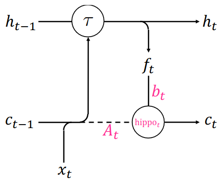
where
- $\mathcal{L}$ is a parametrized linear function
- $\tau$ is any RNN update function
- $[\cdot, \cdot]$ denotes concatenation
- $A_t, B_t$ are fixed matrices depending on the chosen measure
- $N$ and $d$ represent the approximation order and hidden state size
pMNIST
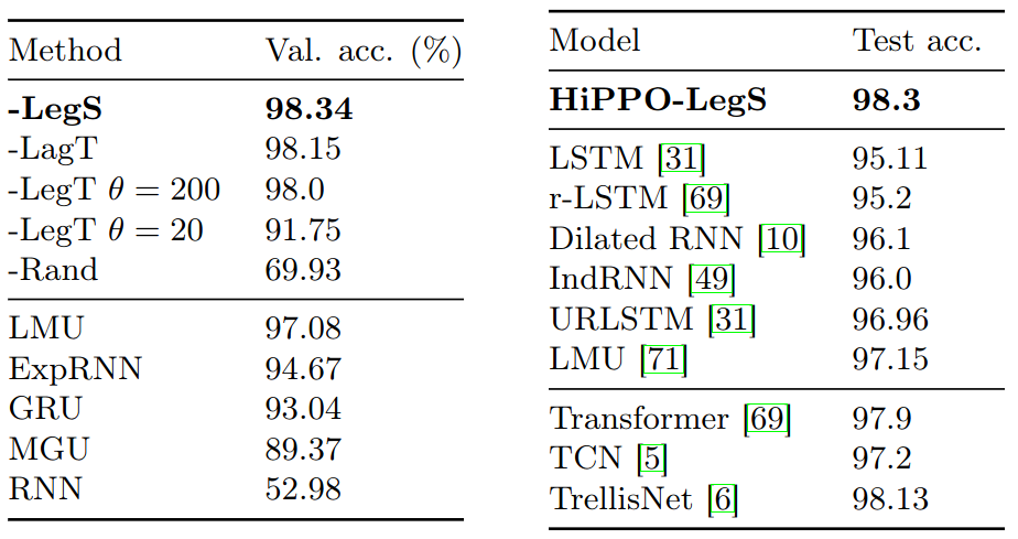
Left: pMNIST validation, average over 3 seeds.
Right: Reported test accuracies from previous works.
Timescale Robustness of HiPPO-LegS
- Why timescale robustness is important?
- Models may be trained on EEG data from one hospital, but deployed at another using instruments with different sampling rates
- Character Trajectories Dataset
- Classify a character from a sequence of pen stroke measurements, collected from one user at a fixed sampling rate
- HiPPO-LegS is timescale invariant, therefore should automatically handle variable sampling rate
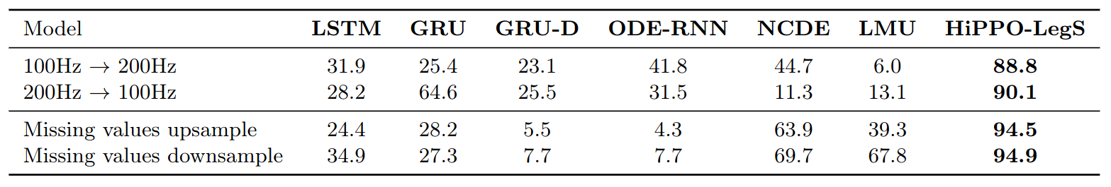
Test set accuracy on Character Trajectory classification on out-of-distribution timescales.
Theoretical Validation and Scalability
Theoretical Validation
- Test if HiPPO-LegS without any additional RNN architecture can memorize history
- Data: random samples from a continuous-time band-limited white noise process, with length $10^6$
- The model is to traverse the input sequence, and then asked to reconstruct the input, while maintaining no more than 256 units in memory
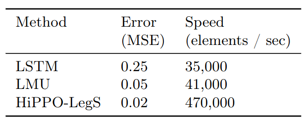
Scalability
- Test training speed
- HiPPO-LegS o is 10x faster than the LSTM and LM