LSSL: Linear State-Space Layer
This post is mainly based on
Overview
- Linear StateSpace Layer (LSSL): $\dot{x} = Ax + Bu$, $y = Cx + Du$
- Recurrent neural networks (RNNs), temporal convolutions (CNNs), and neural differential equations (NDEs) are closely related to LSSL models
- Trainable subset of structured matrices $A$ that endow LSSLs with long-range memory
- Results
- Outperform SOTA by over 10% accuracy on sequential CIFAR
- 80% reduction in RMSE on a 4000-step healthcare dataset compared to benchmark
- On length-16000 speech classification dataset
- Outperforms SOTA by over 20 accuracy points in 1/5 the training time
- Outperforms hand-crafted features
3 Paradigms
| Model Family | Strength | Weakness |
| RNN | Constant computation/storage per time step | 1. Slow to train 2. Optimization difficulties / “vanishing gradient problem” |
| CNN | Fast, parallelizable training | 1. Not sequential / expensive inference 2. Limitation on the context length |
| NDE | Strong theoretical base for continuous-time problems and long-term dependencies | Very inefficient |
Ideally, a model family should combine the strengths of these paradigms, providing properties like parallelizable training (CNN), stateful inference (RNN) and time-scale adaptation (NDE).
However, combining model families should come at the price of reduced expressivity: intuitively, a family that is both convolutional and recurrent should be more restrictive than either.
LSSL
Goal of LSSL: combining 3 paradigms while preserving their strengths
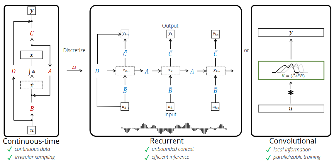
LSSL maps a 1-dimensional function or sequence $u(t) \to y(t)$ through an implicit state $x(t)$ by simulating a linear continuous-time state-space representation in discrete-time.
The linear continuous-time state-space representation is:
\[\dot{x}(t) = Ax(t) + Bu(t)\] \[y(t) = Cx(t) + Du(t)\]where
- $A$: controls the evolution of the system
- $B, C, D$: projection parameters
Connection between LSSL and 3 paradigms
- Recurrent
- If a discrete step-size $\Delta t$ is specified, the LSSL can be discretized into a linear recurrence using standard techniques
- LSSL can be simulated during inference as a stateful recurrent model with constant memory and computation per time step
- Convolutional
- The linear time-invariant systems defined by above are known to be explicitly representable as a continuous convolution
- The discrete-time version can be parallelized during training using convolutions
- Continuous-time
- The LSSL itself is a differential equation
- LTTL can perform unique applications of continuous-time models, such as simulating continuous processes, handling missing data, and adapting to different timescales
Although combining model families should come at the price of reduced expressivity, the authors show the surprising result: LSSLs do not sacrifice expressivity when generalizing CNNs and RNNs
- Classical results from control theory imply that all 1-D convolutional kernels can be approximated by an LSSL (Linear state-space control systems, 2007)
- Two results relating RNNs and ODEs
- Showing that some RNN architectural heuristics (such as gating mechanisms) are related to the step-size $\Delta t$ and can actually be derived from ODE approximations
- Showing that popular RNN methods are special cases of LSSLs
LSSL’s Limitations and Alleviations
Limitations
- Both RNNs and CNNs are weak at remembering long dependencies
- Choosing the state matrix $A$ and timescale $\Delta t$ appropriately are critical to their performance, yet learning them is computationally infeasible
Alleviations
- Specializing LSSLs using a class of structured matrices $A$ to address both challenges mentioned above
- These matrices generalize prior work on continuous-time memory / HiPPO and mathematically capture long dependencies with respect to a learnable family of measures
- These matrices $A$ can be theoretically sped up under certain computation models, even while learning the measure $A$ and timescale $\Delta t$
Backgrounds
ODE Approximation
Any differential equation $\dot{x}(t) = f(t, x(t))$ has an equivalent integral equation
\[x(t) = x(t_0) + \int_{t_0}^t f(s, x(s)) ds\]\(x(t)\) can be numerically solved by Picard Iteration
\[x_{i+1}(t) = x_i(t_0) + \int_{t_0}^t f(s, x_i(s)) ds\]A Concrete Example of Picard Iteration
Suppose we have a first-order ODE:
\[\frac{dx}{dt} = f(t, x) = tx\]with an initial condition:
\[x(0)=1\]Starting from an initial guess for $x(t)$:
\[x_0(t)=1\]Now compute the integral equation:
\[x_1(t) = x_0(t) + \int_0^t f(s, x_0(s)) ds = x_0(t) + \int_0^t s \cdot 1 ds = 1 + \frac{t^2}{2}\]To compute $x_2(t)$, compute the integral equation with $x_1(t)$:
\[x_2(t) = x_1(t) + \int_{t_0}^t s \cdot (1 + \frac{s^2}{2}) ds = 1 + \frac{t^2}{2} + \frac{t^4}{8}\]The result of Picard Iteration on the above problem is a series of functions:
\[\left( 1, 1+\frac{t^2}{2}, 1 + \frac{t^2}{2} + \frac{t^4}{8}, 1 + \frac{t^2}{2} + \frac{t^4}{8} + \frac{t^6}{48}, ... \right)\]that converges to the ground truth solution $x(t)$.
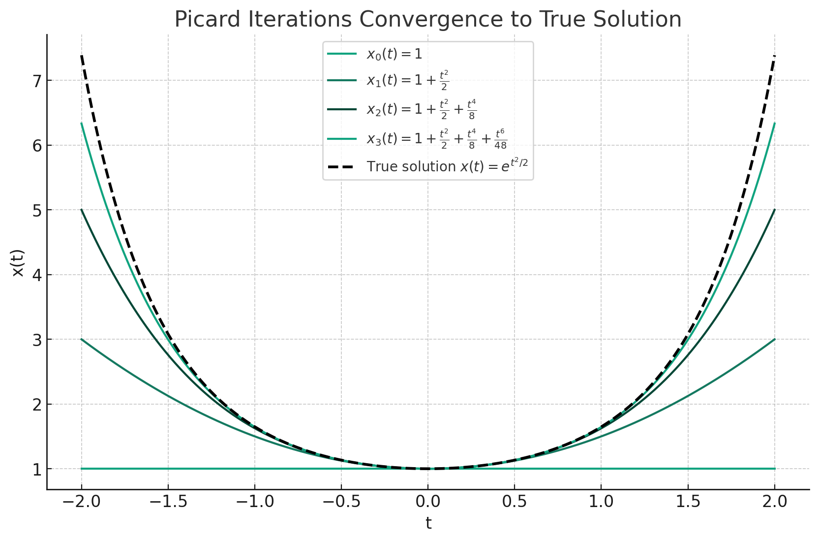
Intuitively, each you compute the integral $\int_{t_0}^t f(s, x_i(s)) ds$, the $x_i(s)$ is off from $x(s)$. Hence the resulting $x_{i+1}(t)$ is different from $x(t)$, but the gap is narrowing.
The convergence is implied by Banach Fixed-Point Theorem and Lipschitz Continuity.
Banach Fixed-Point Theorem
- In a complete metric space, a contraction mapping will have exactly one fixed point, and iterative applications of the contraction mapping will converge to that fixed point
- For Picard iterations, under the right conditions, the mapping from $x_i(t) \to x_{i+1}(t)$ is a contraction
Lipschitz Continuity
- A key condition for the Picard iteration process to work as a contraction mapping
- Intuitively, the function $f(t,x)$ does not change too rapidly with respect to $x$
A function $f(t, x)$ is said to be Lipschitz continuous if there exists a constant LLL (known as the Lipschitz constant) such that for every pair of points $(t, x_1)$ and $(t, x_2)$, the following inequality holds:
\[\|f(t, x_1) - f(t, x_2)\| \leq L\|x_1 - x_2\|\]ODE Discretization
For a desired sequence of discrete times $t_i$, approximations to $x(t_0), x(t_1), …$ can be found by iterating the equation
\[x(t_{i+1}) = x(t_i) + \int_{t_i}^{t_{i+1}} f(s, x(s)) ds\]The generalized bilinear transform (GBT) is specialized to linear ODEs of the form $\dot{x}(t) = Ax(t) + Bu(t)$. Given a step size $\Delta t$, the GBT update is:
\[x(t + \Delta t) = (I - \alpha \Delta t \cdot A)^{-1}(I + (1 - \alpha)\Delta \cdot A)x(t) + \Delta t(I - \alpha \Delta t \cdot A)^{-1} B \cdot u(t)\]Setting $\alpha$ to different values yields different approximation methods:
- $\alpha=0$: classic Euler method
- $\alpha=1$: backward Euler method
- $\alpha=\frac{1}{2}$: bilinear method (better stability)
The author show that the backward Euler method and Picard iteration are actually related to RNNs.
LSSL use bilinear method to compute discrete-time approximations of continuous-time models:
\[\begin{align*} x_t &= \bar{A} x_{t-1} + \bar{B} u_t \\ y_t &= C x_t + D u_t \end{align*}\]where $\bar{A}, \bar{B}$ are computed from GBT update equation above.
Choice of $\Delta t$
In most models, the length of dependencies they can capture is roughly proportional to \(\frac{1}{\Delta t}\) and most ODE-based RNN models have it as an important and non-trainable hyperparameter.
The author show that (paper’s Section 3.2):
- The gating mechanism of classical RNNs is a version of learning $\Delta t$
- The timescale $\Delta t$ can be viewed as controlling the width of the convolution kernel
Ideally, all ODE-based sequence models would be able to automatically learn the proper timescales
HiPPO / Continuous-Time Memory
Consider
- An input function $u(t)$
- A fixed probability measure $\omega(t)$
- A sequence of $N$ basis functions such as polynomials
At every time $t$, the history of $u$ before time $t$ can be projected onto this basis, which yields a vector of coefficients $x(t) \in \mathbb{R}^N$ that represents an optimal approximation of the history of $u$ with respect to the provided measure $\omega$.
The map taking the function $u(t) \in \mathbb{R}$ to coefficients $x(t) \in \mathbb{R}^N$ is called the High-Order Polynomial Projection Operator (HiPPO) with respect to the measure $\omega$.
In special cases of
- Uniform measure $\omega = \mathbb{I}{[0, 1]}$
- exponentially-decaying measure $\omega(t) = \exp(−t)$
$x(t)$ satisfies a differential equation $\dot{x}(t) = A(t)x(t) + B(t)u(t)$ and there exists a closed forms for the matrix $A$.
For more details, see this post.
Linear State-Space Layers
Different Views of the LSSL
Given a fixed state space representation $A, B, C, D$, an LSSL is the sequence-to-sequence mapping defined by discretizing the linear state-space model:
\[\dot{x}(t) = Ax(t) + Bu(t)\] \[y(t) = Cx(t) + Du(t)\]An LSSL has parameters $A, B, C, D, \Delta t$. It operates on an input $u \in \mathbb{R}^{L \times H}$ where:
- $L$: sequence length
- $H$: feature vector dimension
Each feature $h \in [H]$ defines
- A sequence: $(u_t^{(h)})_{t \in [L]}$
- A timescale: $\Delta t_h$
- An output: $y^{(h)} \in \mathbb{R}^L$
where $u^{(h)}$ and $y^{(h)}$ are governed by the discretized state-space model:
\[\begin{align*} x_t &= \bar{A} x_{t-1} + \bar{B} u_t \\ y_t &= C x_t + D u_t \end{align*}\]Computationally, the discrete-time LSSL can be viewed in multiple ways:
Recurrence
The recurrent state $x_{t−1} \in \mathbb{R}^{H \times N}$ carries the context of all inputs before time $t$. The update rule is specified by the discretized state-space model.
Convolution
Let the initial state be $x_{−1} = 0$, then the discretized state-space model’s recurrent update rule yields:
\[y_k = C(\bar{A}^k)\bar{B} u_0 + C(\bar{A}^{k-1})\bar{B}u_1 + ... + C\bar{A}\bar{B}u_{k-1} + \bar{B}u_k + Du_k\]Then $y$ can be computed from the convolution: $y = \mathcal{K}_L(\bar{A},\bar{B},C) * u + Du$, where the kernel $\mathcal{K}_L(\bar{A},\bar{B},C)$ is defined as:
\[\mathcal{K}_L(A,B,C) = (C(A^iB))_{i \in L} \in \mathbb{R}^L = (CB, CAB, ..., CA^{L-1}B)\]Hence, LSSL can be viewed as a convolutional model where the entire output $y \in \mathbb{R}^{H \times L}$ can be computed at once by a convolution:
Limitations
- To train an LSSL, the matrix $\bar{A}$ needs to be updated
- For Recurrence View, compute the discretized state matrix $\bar{A}$ from $A$ requires matrix inversion
- For Convolution View, the Krylov function $\mathcal{K}_L$ require powering $\bar{A}$ up $L$ times
- The computation cost is infeasible in practice
Expressivity of LSSL
Questions to Answer
- While linear recurrences can be unrolled into a convolution, it is not obvious if convolutions can be rolled into by recurrences
- Popular RNN models contains nonlinear activation between each time step, it is not obvious if linear recurrences have the same level of expressivty
Convolutions are LSSLs
State-space systems can be expressed by a convolution:
\[y(t) = \int h(\tau)u(t − \tau) d \tau\]where $h(\cdot)$ is impulse response
A convolutional filter $h$ that is a rational function of degree $N$ can be represented by a state-space model of size $N$. Thus, $h$ can be approximated by a rational function (e.g., by Padé approximants) and represented by an LSSL.
[TBD…]
RNNs are LSSLs
Lemma 3.1
A (1-D) gated recurrence $x_t = (1 - \sigma(z))x_{t−1} + \sigma(z)u_t$, where $\sigma$ is the sigmoid function and $z$ is an arbitrary expression, can be viewed as the $GBT(\alpha = 1)$ (i.e., backwards-Euler) discretization of a 1-D linear ODE $\dot{x}(t) = -x(t) + u(t)$.
Takeaways
- Approximating continuous systems using discretization
- Gating mechanism of RNNs is the analog of a step size or timescale $\Delta t$.
Lemma 3.2
(Infinitely) deep stacked LSSL layers of order $N = 1$ with position-wise non-linear functions can approximate any non-linear ODE $\dot{x}(t) = -x + f(t, x(t))$
Takeaways
- RNN is equivalent to approximate a continuous systems using Picard iteration
- Each layer of a deep linear RNN can be viewed as successive Picard iterates $x_0(t), x_1(t), …$ approximating a function $x(t)$ defined by a non-linear ODE
- We do not lose modeling power by using linear instead of non-linear recurrences, and that the nonlinearity can instead be “moved” to the depth direction of deep neural networks to improve speed without sacrificing expressivity
Check paper Appendix C for details.
Deep LSSLs
- A state-space model can handle 1 feature
- In LSSL, each feature is learned independently, resulting in $H$ different versions of a 1D LSSL processing each of the input features independently
- Full architecture details are described in Appendix B
- Initialization of $A$ and $\Delta t$
- Computational details
- Other architectural details
LSSLs + Continuous-time Memorization
Incorporating Long Dependencies into LSSLs
Issues with recurrent state update matrix $\bar{A}$
- Repeated multiplication by $\bar{A}$ could suffer from the vanishing gradients problem
- Empirically, LSSLs with random matrices $A$ are not effective as a generic sequence model
However, one advantage of continuous-time models is that they are theoretically analyzable:
Theorem 1 (Informal). For an arbitrary measure $\omega$, the optimal memorization operator $hippo(\omega)$ has the form
\[\dot{x}(t) = Ax(t) + Bu(t)\]for a low recurrence-width (LRW) state matrix $A$. Note that LRW matrices are a type of structured matrix that have linear MVM (matrix-vector multiplication).
Theorem 1 tells us:
- $A$ within a particular class of structured matrices implies continuous-time memorization
- Ideally, we would be able to automatically learn the best $A$ within this class of structured matrices
Theoretically Efficient Algorithms for the LSSL
- $A$ and $\Delta t$ are not feasible to train in a naive LSSL
Theorem 2. For any k-quasiseparable matrix $A$ (with constant $k$) and arbitrary $B$, $C$, the Krylov function $\mathcal{K}_L(A, B, C)$ can be computed in quasi-linear time and space $O(N + L)$ and logarithmic depth (i.e., is parallelizable). The operation count is in an exact arithmetic model, not accounting for bit complexity or numerical stability.
Theorem 2 tells us:
- However, for any k-quasiseparable matrices $A$, the Krylov function $\mathcal{K}_L(A, B, C)$ can be computed in near linear time
- LSSL can be efficiently trained for some special $A$, although the implementation could be complicated
Experiments
Models
- Baselines
- CKConv: continuous convolution kernel
- UnICORNN: ODE-inspired RNNs
- NCDE/NRDE: Neural Controlled/Rough Differential Equations
- LSSL
- LSSL-f: $A$ matrix is fixed to one of the HiPPO matrices
- LSSL: $A$ matrix is trainable
LSSL Implementation
- Model architecture
- See Appendix B.4
- Initialization
- $A$: follows HiPPO-LegS
- $\Delta t$
- Log-uniform in range $(\Delta t_{min}$, $\Delta t_{max})$.
- $\Delta t_{min}$, $\Delta t_{max}$ were generally 100x apart to contain length of sequences in the dataset
- Training
- Train at much higher learning rates
- Not sensitive to hyperparameter
- Light tuning primarily on learning rate and dropout
- No weight decay, gradient clipping, weight norm, input dropout, etc.
- How $\Delta t$ is learned?
- See Appendix E.3, E.3.1, E.3.2
Image and Time Series Benchmarks
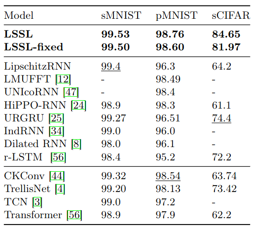
Pixel-by-pixel image classification. LSSL outperforms SoTA on sCIFAR by more than 10 points. All results were achieved with at least 5x fewer parameters than the previous SoTA.
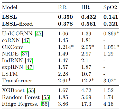
Vital signs prediction on the BDIMC healthcare datasets (length 4000 time series regression problems). RMSE for predicting respiratory rate (RR), heart rate (HR), and blood oxygen (SpO2). LSSL reduces RMSE by more than two-thirds on all datasets.
Speech and CelebA
Both dataset contains very long time series.
Speech
- Speech Commands (SC) dataset: classification of 16000-length series (1s@16kHz)
- Results
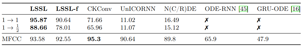
- On raw signal: LSSL and LSSL-f significantly outperform SOTA
- On MFCC: LSSL and LSSL-f are SOTA competitive
- Relationship with MFCC
- MFCC extracts sliding window frequency coefficients (mapped fourier transform coefficients)
- LSSL may be interpreted as automatically learning MFCC-type features, using Legendre basis rather than trigonometric basis
CelebA
- CelebA dataset: classification of 4 facial attribute on 38000-length series ($178 \times 218$ pixel image)
- Results
- ResNet-18 competitive with 1/10 of parameters
- First generic sequence model to achieve ResNet competitive performance
Advantages
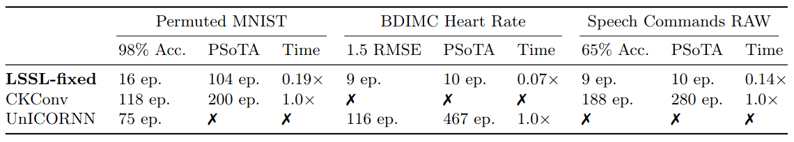
Convergence Speed
- Parallelizable in convolutional view
- Both sample (measured by epochs) or computational (measured by wall clock) efficient
- LSSLs reached the target in a fraction of the time of SOTA model
Timescale Adaptation
- LSSL can effectively handle missing data or sampling rate shift in time series
- LSSLs can perform timescale adaptation at inference time (1/2 of training sampling rate), and still outperforming the SOTA with no shift
LSSL Ablations
- Findings
- $\Delta t$ and $A$ are critical to the performance of these continuous-time models
- Learning $\Delta t$ adds only $O(H)$ parameters
- Learning $A$ adds $O(N)$ parameters
- Learning both adds less than 1% parameters compared to the base models with $O(HN)$ parameters
Memory dynamics $A$
- Consistent increase in performance from LSSL-f to LSSL
- Incorporating the theory of Theorem 1 is necessary for LSSLs
- Training $A$ can be interpreted as learning the measure for memorization
Timescale $\Delta t$
- Previous ODE-based RNN models cannot learn $\Delta t$
- LSSL’s ability to learn $\Delta t$ is its direct generalization of the gating mechanism of RNNs
- Learning $\Delta$ is important: on sCIFAR, LSSL-f with poorly-specified $\Delta t$ gets only 49.3% accuracy
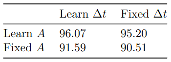
Learning $\Delta t$ alone provides an orthogonal boost to learning A.
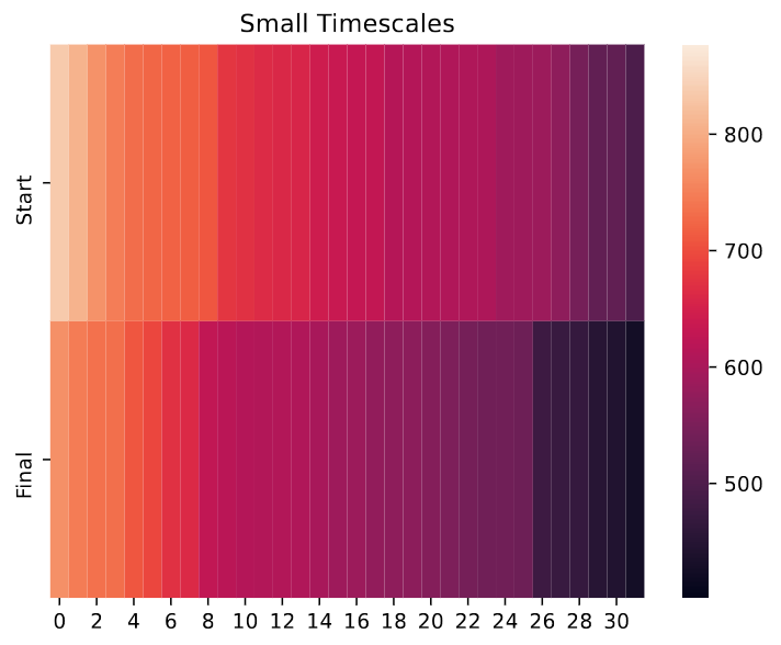
Comparing 32 smallest $\Delta t$ values at the start and end of training for the first layer of LSSL model on the Speech Commands Raw dataset. The plots visualize $\frac{1}{\Delta t}$. which can be interpreted as the timescale at which they operate. LSSL modify the $\Delta t$ to more appropriately model the speech data.
Limitations of LSSL
- Theorem 2’s algorithm is sophisticated, not numerically stable and thus not usable on hardware
- Thus Theorem 2’s contributions are limit to a proof-of-concept fast algorithms
- Whether fast, numerically stable, and practical algorithms for the LSSL exist is an open question
- Space inefficient
- LSSL uses $O(NL)$ instead of $O(L)$ space
- $L$: 1D sequence of length
- $N$: latent state representation of dimension
- Future work (S4) provided a new parameterization and algorithms for state spaces