Temporal Convolutional Network
This post is mainly based on
- WaveNet: A Generative Model for Raw Audio, 2016
- An Empirical Evaluation of Generic Convolutional and Recurrent Networks for Sequence Modeling, 2018
- Blog: Temporal Convolutional Networks and Forecasting
Temporal Convolutional Network is an alternative architecture to Recurrent Neural Network (RNN) in sequence modelling task. TCN can handle variable length input and can be configured to into different receptive fields. Unlike RNN, TCN can be easily parallelized.
The architecture was proposed as time delay neural network nearly 30 years ago and a more complex version of TCN was recently used in the 2016 WaveNet paper. The 2018 paper formalized the definition of TCN and conducted ablation studies to compare it against RNN cross a diverse range of tasks and datasets.
The term “Temporal Convolutional Network” is first used in the 2016 paper. Reader may want to distinguish the TCN described in the 2018 paper from the 2016 paper since they are different architectures. My understanding is that, the 2016 paper’s convolution is non-causal and the goal of the architecture is to perform segmentation in time series, which can be viewed as a 1-dimensional U-Net.
Assumptions
Consider the sequence modelling task: $((x_1, x_2, …, x_T), (y_1, y_2, …, y_T))$. The goal is to find some mapping $f: \mathcal{X}^T \rightarrow \mathcal{Y}$, where
\[\hat{y}_t = f(x_0, ...,x_t)\]This is called a causal constraint: $y_t$ only depends on past data: $x_1, …, x_t$ and not depends on future data: $x_{t+1}, x_{t+2}, …$.
The optimization goal is to minimize some loss between observed and prediction:
\[L( (y_0, ..., y_T), (\hat{y}_0, ... \hat{y}_T) )\]Causal Convolutions
Causal Convolution satisfies the following two properties:
- Output length $\hat{y}_1, …, \hat{y}_T$ is equal to input length $x_1, …, x_T$
- No leakage of future information into the past $ \hat{y}_t = f(x_0, …,x_t) $
For a convolution filter with kernel size $k$, causal convolutions can be achieved by
- Left padding the sequence by $k-1$
- Pass the padded sequence through the convolution filter
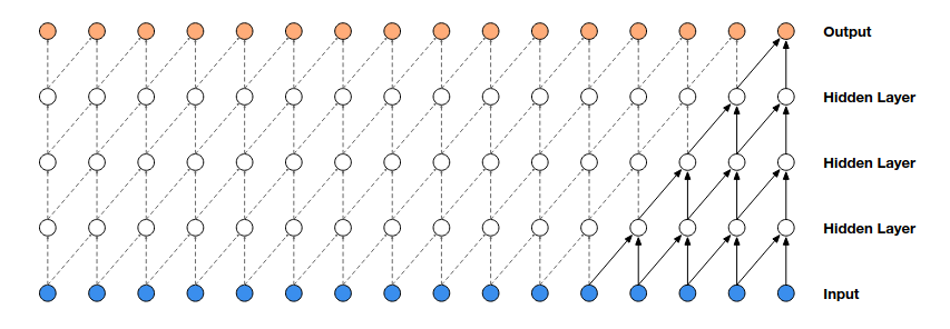
A vanilla causal convolution’s receptive field grows linearly w.r.t. depth and kernel size. Hence, long range dependency requires either large filters or many layers, which renders the optimization problem hard.
Dilated Causal Convolution
Dilated causal convolution $f$ is a causal convolution filter with filter size $k$ and dilation factor $d$:
\[f(x_1, ...., x_t) = \sum_{i=0}^{k-1} f(i) \cdot x_{t - d \cdot i}\]where $f(i)$ is the $i$-th weight of the conv filter, and $t - d \cdot i$ specifies the index of the input sequence $x$ correspond to the $i$-th weight. Note that dilation is different from stride: A conv filter with stride $d$ still has linear receptive field, whereas a conv filter with dilation $d$ has exponential receptive field. When $d = 1$, a dilated convolution reduces to a regular convolution.
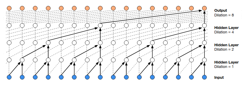
The receptive field of a dilated causal convolution is $(k-1)d$.
We typically increase $d$ exponentially w.r.t. depth, which ensures that the receptive fields of the 1st layer does not overlap each other and there is no gap between adjacent receptive fields, as shown in the figure above.
Residual Connections
A TCN can be constructed in regular blocks or residual blocks. For deeper networks, the residual connection reduce the difficulty of the optimization problem.
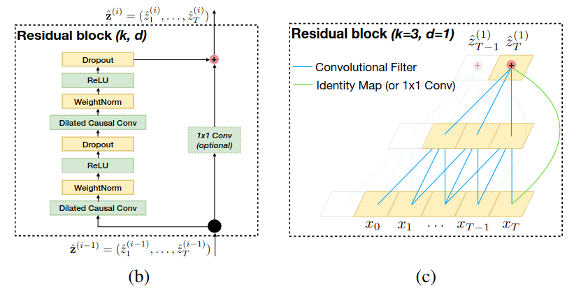
Detailed configuration of the residual block
- Two layers of dilated causal convolution + ReLU activation + Dropout
- Weight normalization: normalizes the weights of the layer, instead of the input mini-batch
- Spatial dropout: drop a whole channel, instead of individual weight parameter
- 1x1 convolution on $x$ to ensure $x$ and $f(x)$ have the same number of channels
- Residual connection $y = x + f(x)$
Discussion on Normalization Layer
- Weight normalization performs poorly on certain tasks (e.g., speech data)
- Consider an input batch $(B, C, T)$, with $B,C,T$ refer to batch, channel, time dimension
- Wav2Vec adopted Layer normalization (normalize across $C, T$)
- Some TCN like encoder uses Batch normalization (normalize across $B, T$)
- In my experiments
- Batch normalization and Instance normalization (normalize on $T$ only) delivers the best result, depending on tasks
- Note that if the modelling task is causal / forecast, any normalization on $T$-dimension will leak information
Properties of TCN
Advantage
- Parallelism
- Flexible receptive field
- Stable gradient
- Low memory requirement during training
- Variable length input
Disadvantage
- High memory requirement during evaluation
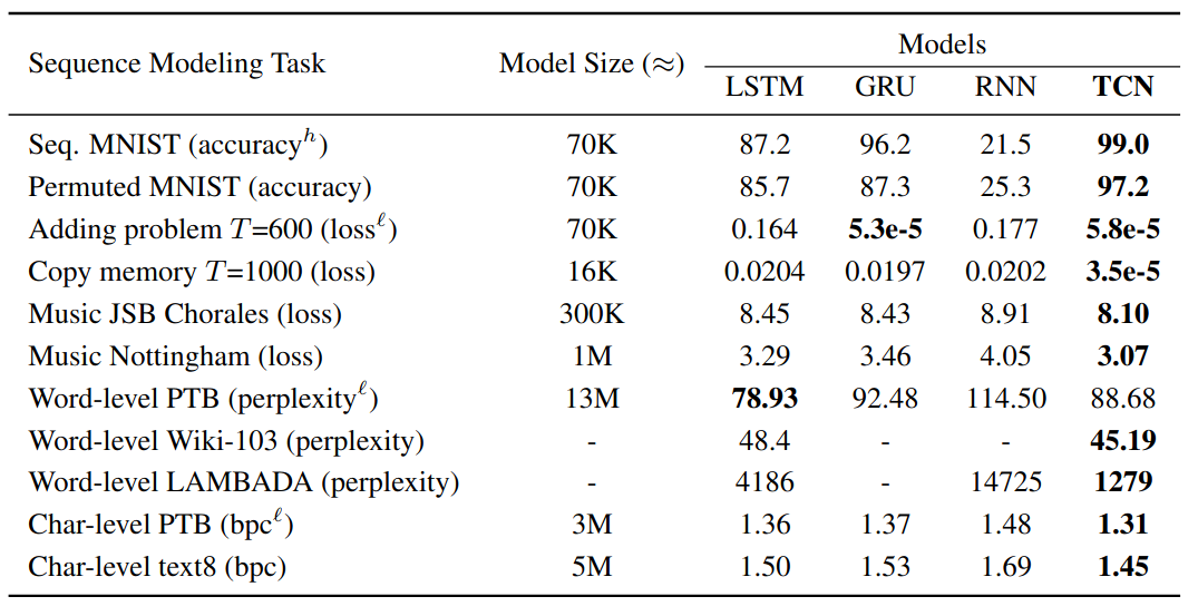
Ablation studies
Evaluation tasks/datasets
- The adding problem: sum a length-n sequence according to the mask
- Sequential MNIST: flattened MNIST image
- P-MNIST: randomly permuted MNIST image
- Copy memory: memorize the 10 values at the beginning and copy it after $T$ steps
- JSB Chorales and Nottingham: polyphonic music dataset
- PennTreebank: character-level and word-level language modeling
- Wikitext-103: word-level language modeling
- LAMBADA: word-level language modeling
- text8: character-level language modeling
Results
Rate of convergence
TCN converge significantly faster than LSTM and GRU on
- The adding problem
- Sequential MNIST
- P-MNIST
- Copy memory