Weight Initialization
This post is mainly based on:
- Understanding the difficulty of training deep feedforward neural networks, AISTATS 2010
- Deep Sparse Rectifier Neural Networks, AISTATS 2011
- Delving Deep into Rectifiers: Surpassing Human-Level Performance on ImageNet Classification, ICCV 2015
- Andre Perunicic’s blog
Literature Review
prior to 2006, deep multilayer neural networks were not successfully trained. Between 2006-2009, research focused on unsupervised pre-training on Deep Belief Networks (DBN). A DBN is a layer wise graphical model, with joint distribution:
\[P (x, g^1, g^2, ... , g^l) = P (x|g^1)P (g^1|g^2) · · · P (g^{l−2}|g^{l−1})P (g^{l−1}, g^l)\]where $x$ is the input, and $g^i$ are the hidden variables at layer $i$. A Restricted Boltzmann Machine (RBM) is the prior $P(g^{l−1}, g^l )$. You can view DBN as stacked RBM. The strategy to train DBN is described in Greedy Layer-Wise Training of Deep Networks. A RBM is different from a feed forward neural network as the connection between RMB is stochastic, $P(g^{l−1}, g^l )$. This post provides a good description of their differences. I don’t have any experience on training RBM, but from my understanding on efficiency of MCMC, if training of each $P (g^{l−1}, g^l )$ relies on Gibbs sampling, the speed should be quite slow.
Perhaps an important reason that DBN fallen out of favor compared to neural network is people figure out how to solve the vanishing gradient problem: compared to stacking one additional layer at a time, training all layers together with gradient descent should be more efficient and easy to implement. The timeline is:
- In 2010, Xavier Glorot and Yoshua Bengio introduced Xavier initialization and find that logistic sigmoid activation is unsuited for deep networks training
- In 2011, Xavier Glorot et al., found that ReLU is more suitable for training of deeper network in the paper Deep Sparse Rectifier Neural Networks
- In 2012, AlexNet was introduced, which features ReLU as activation function
- In 2015, Kaiming He published Kaiming initialization
Tanh and Xavier initialization
Notations
We will use the notation from Andre Perunicic’s blog and Glorot’s paper. Consider a feed forward network,
\[x^{(0)} \xrightarrow {W^{(0)}} \underbrace{\left( s^{(0)} \xrightarrow{f} x^{(1)} \right)}_{\text{Hidden Layer 1}} \xrightarrow{W^{(1)}} \ldots \xrightarrow{W^{(M-1)}} \underbrace{\left( s^{(M-1)} \xrightarrow{f} x^{(M)} \right)}_{\text{Hidden Layer M}} \xrightarrow{W^{(M)}} \underbrace{ \left( s^{(M)} \xrightarrow{\sigma} \sigma(s^{(M)}) \right) }_{\text{Output Layer}}\]where $x^{(i)}$ is the input vector of i-th hidden layer, $s^{(i)}$ is the vector before activation, $W^{(i)}$ is the linear transformation $s^{(i)} = x^{(i)} W^{(i)}$, and $x^{(i+1)}$ is the output vector after activation.
The gradient on $w$ can be computed using reverse mode AD:
\[\frac{\partial L}{\partial w_{jk}^{(i)}} = \frac{\partial L}{\partial x_k^{(i+1)}} \frac{\partial x_k^{(i+1)}}{\partial w_{jk}^{(i)}}\]Assume we know how to compute the first term $\frac{\partial L}{\partial x_k^{(i+1)}}$ (just an induction from base case), the second term $\frac{\partial x_k^{(i+1)}}{\partial w_{jk}^{(i)}}$ can be computed as:
\[\begin{align*} \frac{\partial{x_k^{(i+1)}}}{\partial w_{jk}^{(i)}} &= \frac{\partial{f(s^{(i)}_j)}}{\partial s_j^{(i)}} \frac{\partial s_j^{(i)}}{\partial w_{jk}^{(i)}} \\ &=f'(s^{(i)}_j)\, x_j^{(i)} \end{align*}\]To avoid exploding or vanishing gradient problem, $f’(s^{(i)}_j)$ and $x_j^{(i)}$ should not be too big or small. Below are three observations:
- Gradient from next layer $\frac{\partial L}{\partial x_k^{(i+1)}}$ should be well behaved
- If activation from previous layer $x_j^{(i)}$ is too big or small, we will exploding or vanishing gradient when the effects are compounded by multiple layers
- For tanh and sigmoid activation, gradient will saturate ($f’(s^{(i)}_j) = 0$) when $s^{(i)}$ is too big or small
Sigmoid vs Tanh
Results are from section 3.1 of Glorot’s paper. The authors conduct experiments on MNIST digits classification. For sigmoid, they found at the beginning of the training, all the sigmoid activation values of the last hidden layer are pushed to their lower saturation value of 0, which causes vanishing gradient. This phenomenon is more server on deeper network.
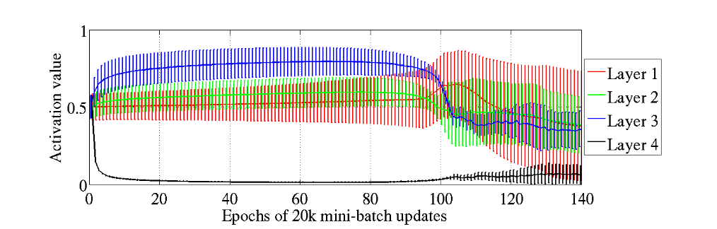 Mean and standard deviation (vertical bars) of the activation values (output of the sigmoid) during supervised learning, for the different hidden layers of a deep architecture. The top hidden layer quickly saturates at 0 (slowing down all learning), but then slowly desaturates around epoch 100.
For tanh, they found no saturation at the beginning, but there is sequentially saturation starting with layer 1 and propagating up in the network.
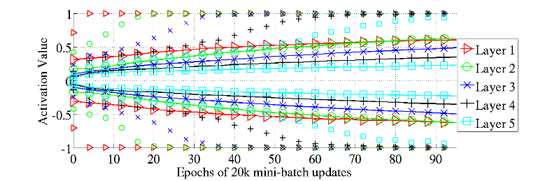 98 percentiles (markers alone) and standard deviation (solid lines with markers) of the distribution of the activation values for the hyperbolic tangent networks in the course of learning. We see the first hidden layer saturating first, then the second, etc.
They proposed a possible explanation of this result: consider the last layer (say, layer 5) of the network. At the beginning of the training, feature output from layer 4 is random and the optimization will push the activation to zero for a lower loss. For tanh, gradient at $x \approx 0$ is 1, which looks good. For sigmoid, gradient at $x \approx 0$ is 0, which result in vanishing gradient in shallower layers.
Loss function
Author found that, compared to L2 loss (they called quadratic cost), negative log likelihood or cross-entropy loss induced better shape on optimization problem of weight $w$. This corresponded to less loss plateaus observed in training of neural network with cross-entropy loss.
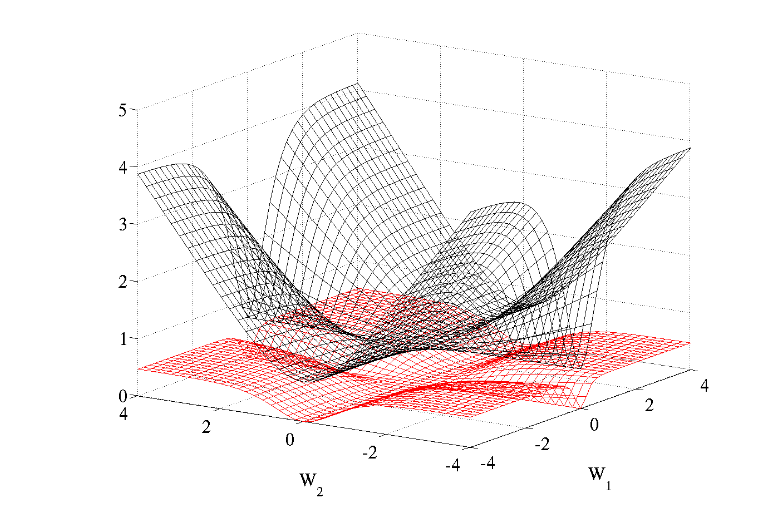 Cross entropy (black, surface on top) and quadratic (red, bottom surface) cost as a function of two weights (one at each layer) of a network with two layers, W1 respectively on the first layer and W2 on the second, output layer.
Xavier initialization
Previous study found that after initialization, back-propagated gradients were smaller as one moves from the output layer towards the input layer. The goal of Xavier initialization is to keep variance of gradient on $s^{(i)}$ constant across multiple layers. We will skip the derivations since they are clearly explained in Andre Perunicic’s blog. The result is:
\[\operatorname{Var}(W_i) = \frac{2}{n_i + n_{i+1}}\]where $n_i$ is number of hidden units on layer i. Given the variance of the uniform distribution, $\operatorname{Var} ( U(-a,a) ) = \frac{a^2}{3}$, we can substitute $\operatorname{Var}(W_i)$ and reach $a = \sqrt{\frac{6}{n_i+n_{i+1}}}$.
ReLU and Kaiming initialization
ReLU
prior to 2010, ReLU is not preferred as an activation function due to hard non-linearity and non-differentiability at zero. In the 2011 paper, authors show that ReLU is a better model of biological neurons and yield equal or better performance than tanh. Their reasons are:
- Neuroscience Observations: ReLU better model biological neurons where they either fire (1) or not fire (0)
- ReLU can naturally output zeros and hence learns sparse representations
Network with ReLU as activation was named Deep Rectifier Networks (I guess back at 2011, activation function is not yet treated as a hyperparameter and this is an important discovery). In experiment section, they first compared ReLU to soft-plus activation, and suggested that non-differentiability at zero does not hurt performance. Second, they compared ReLU to tanh and result showed that ReLU yield better convergence on CV and NLP (sentiment analysis) tasks.
Although ReLU is widely used in practice, there are areas where tanh activation is preferred. For example, tanh is heavily used RNN, LSTM and GRU. I am not able to find formal discussions on this topics, but this post offers some empirical results. Tanh is also widely used in some control problems, e.g., policy network of actor-critic learning in reinforcement learning.
Kaiming initialization
In the 2015 paper, the authors Parametric ReLU and a proper initialization for ReLU. They pointed out that Xavier initialization is based on the assumption that activations is linear, which is invalid for ReLU. At the step
\[\operatorname{Var}(s_i) = n_i \operatorname{Var}(w_i x_i) = n_i \operatorname{Var}(w_i)\operatorname{Var}(x_i)\]Assume $s_{i−1}$ have a symmetric distribution around zero. Due to $x_i = \operatorname{ReLU}(s_{i-1})$, half of variance is chop out by the ReLU operator: $\operatorname{Var}(x_i) = \frac{1}{2}\operatorname{Var}(s_{i-1})$. This leads to:
\[\operatorname{Var}(w_i) = \frac{2}{n_i}\]Therefore, for a normal $w_i$, the std is $\sqrt{2/n_i}$. For a uniform $w_l$, the std is $\sqrt{\frac{6}{n_i}}$. This result is consistent with Keras documentation, but differs by a factor of $\sqrt{2}$ with PyTorch documentation.
Experiments
Please refer to this repo.