Ensemble Learning
This post compares different ensemble learning algorithms and is mainly based on
- Greedy function approximation: A gradient boosting machine, 2001
- XGBoost: A Scalable Tree Boosting System, 2016
- LightGBM: A Highly Efficient Gradient Boosting Decision Tree, 2017
Bagging
Bagging is the abbreviation of the term bootstrap aggregating. It is commonly applied to weak learners like decision tree. The goal is to reduce variance. Bagging is a special case of the model averaging and is generally parallelizable.
Data Bagging
Also called bootstrap aggregating. Bagging create $m$ dataset $D_1, …, D_m$ by sampling the original dataset with replacement and build weak learners $f_i$ on top of each $D_i$. The final output is an average over $f_i$.
Feature Bagging / Random Forest
Random Forest can be viewed as feature bagging: at the split step, the random forest algorithm sample $m$ subsets of features $X_1, …, X_m$ and build weak learners $f_i$ on top of them. The final output is an average over $f_i$.
There is an well written blog on feature importance mechanism in Random Forest.
Boosting
Boosting is used to combine weak learners into strong ones. The first boosting algorithm was called a 3-stage booster and was proposed by Robert Schapire in 1990 under the PAC learning framework. A detailed discussion can be found in this post. In 1995, the 3-stage booster was extended to Adaboost algorithm. Adaboost avoids recursive calls and fits better to the “learning under a fix dataset” framework (vs online learning with a data oracle). Adaboost combines weak learners by training them under different distributions/weights and taking a weighted majority vote. A detailed discussion can be found in this post and an intuitive walk through can be found here.
Gradient Boosting
The gradient boosting algorithm is more complex compared to Adaboost and requires some understanding of optimization.
Let $L(\cdot, \cdot)$ be a differentiable loss function and \(\{ (x_i, y_i) \}_{i=1}^N\) be a dataset. At round $m$, Gradient boosting construct strong learner $F_m$ by adding a weak learner on top of the previous learner: $F_m = F_{m-1} + f_m$ . To obtain $f_m$, gradient boosting compute the gradient $\nabla_i$ of the loss function $L(y_i, F_{m-1}(x_i))$ with respect to $F_{m-1}$. The resulting $\nabla_i$ is a scalar. A weak learner $f_m$ is fitted to the dataset \(\{ (x_i, -\nabla_i) \}_{i=1}^N\) to estimate the negative gradient. Following the gradient descent (GD) framework, we can set a learning rate $\rho$ and add $-\rho \cdot \nabla_m$ in each GD step, to minimize the loss function $L$, where $-\nabla_m$ is estimated by the weak learner $f_m$.
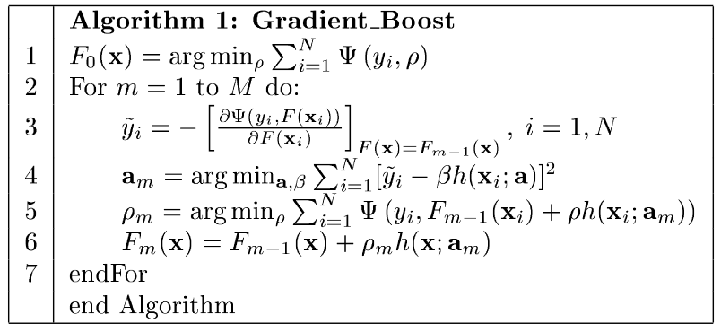
A detailed discussion over the similarity between gradient boosting and numerical optimization in function space can be found in the original paper. The paper also used a variable learning rate $\rho_m$, which is searched at each round $m$ (I think this is not common in modern implementations as most of them uses a fixed learning rate). The notation in the paper is a bit confusion:
- $\Psi(\cdot, \cdot)$: loss function
- $\rho$ in the first line: initial prediction, $\rho \in \mathbb{R}$
- $h(x;a)$: weak learner, where $a$ are the parameters of $h$
- $\beta, \rho$: learning rate search parameter
- $\rho_m$: optimal learning rate at round $m$
The gradient boosting algorithm is as follow:
An Example
Under the regression framework, if we set the loss function $L = \frac{1}{2}(y - \hat{y})^2$. Then the negative gradient w.r.t to $\hat{y}$ is $- \nabla L = y - \hat{y}$. At each round, we fit $f_m$ to the residual $y - F_{m-1}$ and add $f_m$ on top of $F_{m-1}$. In other words, each subsequent regression model correct the mistakes made by the previous combined model, resulting in boost of accuracy.
If we compare Adaboost and gradient boosting under this framework:
- Assume the ground truth function is $f$
- Adaboost
- Output of each weak classifier $f_m$ is “correct” under the weighted distribution \(\mathcal{D}_m\)
- $\mathbb{E}_{\mathcal{D}_m}[f_m(x)] = f(x)$
- Gradient Boosting
- Output of each weak classifier $f_m$ should to be added on top of $F_{m-1}$
- $\mathbb{E}[F_m(x)] = f(x)$, where $F_m(x) = F_{m-1}(x) + f_m(x)$
For classification problems, $L = -\sum_{k=1}^K y_k \log p_k(x)$ and $\nabla = y_k - p_k(x)$, where $k$ is the index of the class. If you prefer an intuitive walk through, good examples can be found here and here.
Weak Learner: Decision Tree
We will take a quick detour to discuss decision tree, since some the optimizations of XGBoost and LightGBM aims to improve tree building efficiency.
There are many algorithms to build a decision tree, the most notable ones are:
- ID3 (Iterative Dichotomiser 3)
- C4.5 (successor of ID3)
- CART (Classification And Regression Tree)
When building decision tree, there are many design choices, for example:
- Should the tree be binary or not?
- How to handel missing data?
- How to prune the tree?
ID3, C4.5 and CART make different design choices:
- C4.5 improves on ID3 by support continuous features and missing data
- CART default to binary split, while ID3 and C4.5 support multiway split
- Split criteria
- ID3: Information gain
- C4.5: Gain ratio
- CART: Ginni index
If you are interested in details, here is a blog and a survey paper. The main takeaways are:
- Decision tree make the split decision based on information gain
- At each step, the decision tree split data into two or more groups
- To compute gain, the algorithm calculate the similarity for data in each group
- Greedy Heuristic
- The algorithm makes local improvement
- At each node, try different splits and choose the split with max gain
You may notice that the above split strategy has an efficiency problem for continuous variables: let $N$ be the size of the dataset $X$ and $X_j$ be a continuous variable with $n_j$ unique values. There are $n_j-1$ ways to split the data: $\{X|X_j < s\}, \{X|X_j >= s\}$. With the “pre-sorted implementation”, we first sort all points with $O(N\log N)$ complexity, then loop through the sorted array compute gain for all splits. The inefficient originate from the fact that we need to try all splits. XGBoost and LightGBM use different strategies to “try less split”:
- XGBoost uses weighted quantile sketch: only try quantiles
- LightGBM uses GOSS: only try “important” points
We will explain the two strategies in details below.
XGBoost
As the title suggested, XGBoost is “A Scalable Tree Boosting System”. XGBoost improves the efficiency on both the algorithmic side and hardware side (cache access patterns, data compression and sharding). We will discuss the algorithmic optimization only.
Regularized Learning Objective
\[L(\phi) = \sum_i L(\hat{y}_i, y_i) + \sum_k \Omega(f_k)\]where \(\Omega(f) = \gamma T + \frac{1}{2} \lambda \| w \|\) is the regularization term; $T$ is number of leave; $w$ is leaf weight for regression tree. This regularization term allow better control over tree pruning.
Gradient Tree Boosting
For the optimization problem, given the loss function at step t:
\[L^{(t)} = \sum_i L(y_i, \hat{y}_i^{(t-1)} + f_t(x_i)) + \Omega(f_t)\]XGBoost use 2nd order estimation (Taylor expansion):
\[L^{(t)} = \sum_i \left[ L(y_i, \hat{y}_i^{(t-1)}) + g_i f_t(x_i) + \frac{1}{2} h_i f_t^2(x_i) \right] + \Omega(f_t)\]where $g_i$ is the gradient and $h_i$ is the hessian for point $i$. However, due to we are taking derivative against a scalar $\hat{y}_i^{(t-1)}$, both $g_i$ and $h_i$ are scalars.
Weighted Quantile Sketch
Goal: reduce the number of split to try on large dataset (on small dataset, XGBoost still uses the “pre-sorted implementation”). The “check all possible split” method discussed above is called exact method in this paper. The paper proposed an approximate method called “Weighted Quantile Sketch”; we will decompose this method into two parts: “Weighted” and “Quantile Sketch”.
The “Quantile Sketch” part propose splits using a histogram with approximate $\frac{1}{\varepsilon}$ bins.
- For the $k$-th feature $x_k$
- Consider a rank function $r_k(x_k)$ which output the quantile of $x_k$
- Propose splits $\{s_{k,1}, s_{k,2}, · · · s_{k,l}\}$
- Adjacent splits should to be close to each other in quantile
The “Weighted” part modify the bin size of histogram. Consider we construct a dataset for feature $k$: \(\mathcal{D}_k = \\{ (x_{i,k}, h_i) \\}_{i = 1}^N\), where \(h_i\) is the second order gradient. The rank function mentioned above is modified to:
\[r_k(z) = \frac{1}{\sum_{(x,h) \in \mathcal{D}_k} h} \sum_{\sum_{(x,h) \in \mathcal{D}_k,x<z} h}\]What the above equation said is: now redefine the quantile computation such that each point has weight $h$, instead of weight $1$ in a regular quantile function. Note that for regression problem, $h=1$ for all $x$. Therefore the weighted quantile is just a normal quantile. However, for binary classification problem, $h$ increase as predicted probability approaching 0.5. This gives the hard-to-classify points more weight and results in smaller bin size. In other words, for hard-to-classify points, the XGBoost algorithm will construct more refined splits in feature $k$. We omit all derivations above and interested readers please refer to the paper.
The paper compared the performance between exact method, applying approximation method just once in each tree, applying approximation method after each split. Refer to Section 3.2, 3.3 and Figure 3 in the paper for more details.
Sparsity-Aware Split
Goal: handle missing data, frequent zero entries or one-hot encoding. The implementation is simple: For a feature $x_k$, consider only non-missing data $I_k$, generate splits using the above mentioned method. For each split $s$, $I_k$ is divided into two sets $L$ and $R$. Try two different grouping: put the entire missing set to $L$, vs, put the entire missing set to $R$. Choose the grouping with the largest gain.
The authors mentioned that compared to a naive implementation, the sparsity-aware split result in a 50x speed improvement in a Kaggle dataset. For details, check the paper’s Section 3.4.
LightGBM
LightGBM further improves the efficiency of gradient boosting. In general, LightGBM is faster than XGBoost. In Section 2.1, the authors analyze the computation complexity of histogram-based algorithm:
- Histogram building: $O(n_{data} \times n_{feature})$
- Split point finding: $O(n_{bin} \times n_{feature})$
Due to $n_{bin} \ll n_{data}$, histogram building dominate the computation cost. If we can reduce $n_{bin}$ or $n_{feature}$, we can significantly improve the efficiency of gradient boosting.
Gradient-based One-Side Sampling (GOSS)
As previously mentioned, LightGBM aims to reduce $O(n_{bin})$ by only try “important” points. The importance of a point is defined as the size of its gradient. The intuition is: “if an instance is associated with a small gradient, the training error for this instance is small and it is already well-trained.” GOSS divide all points into two sets: large gradient set $A$ and the rest $B$. All points in $A$ and a random sample of $B$ is passed to the tree building algorithm, reducing $n_{data}$. We omit details like “assigning weight to points in $B$” and error analysis; interested reader please refer to Section 3 of the paper.
Exclusive Feature Bundling (EFB)
To reduce $n_{feature}$, the authors proposed EFB combine multiple features into one feature. The motivation is that high-dimensional data are usually very sparse and many features could be mutually exclusive (an extreme case is a one-hot encoded categorical variable with many unique values). The feature bundle problem could be reduced to the graph coloring problem (NP-Hard) and approximated by a greedy algorithm with $O(n_{feature}^2)$ complexity (only need to run once). For details, please refer to Section 4 of the paper.
XGBoost vs LightGBM
The two algorithms also have different tree growth strategy: XGBoost adopts a level-wise growth strategy to produce balanced trees; LightGBM uses leaf-wise growth strategy which choose the leaf with max delta loss to grow (Section 5.1 of LightGBM paper). This produce imbalanced trees.
A good comparison between the two algorithm can be found here