AdaBoost
This post is mainly based on
The full name for AdaBoost is Adaptive Boosting. Following the work of 3-stage boosting in 1990, Robert Schapire and Yoav Freund proposed AdaBoost in 1995 in the paper A Decision-Theoretic Generalization of On-Line Learning and an Application to Boosting. Compared to 3-stage boosting, the AdaBoost is different in the following ways:
- Change of learning setting
- 3-stage boosting assumes access to an example oracle
- AdaBoost operate on a fixed training set
- AdaBoost’s assumption is more closed to most machine learning application’s setting
- No longer requires compounding of weaker learners
- To construct strong learners, you need to compound 3-stage boosters (This could be hard to implement in practice)
- AdaBoosting uses weighted sum of weaker learners to construct strong learners
- Implementation only requires a simple loop
- The algorithm is “adaptive” since it can take advantage of better learners in intermediate steps and assign higher weights to better learners
The high level idea of Adaboost is the same as 3-stage boosting: given $h_t, \mathcal{D}_t$, construct $ \mathcal{D}_{t+1} $ s.t. $P(\text{error of } h_t \text{ under } \mathcal{D}_{t+1}) = 0.5$. To achieve this, weights on misclassified examples at stage $t$ need to be increased, prioritizing the weaker learner to those misclassified examples in the next stage $t+1$.
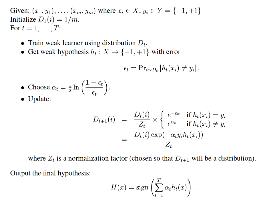
Algorithm
Reference:
Note that “weight on sample” and “reweighing distribution” are equivalent, as some articles describe the algorithm as “adjusting weight on samples”. If you look at the loss function for the learner, the weight on sample $w_i$ is equivalent to sampling probability $p(x_i)$.
Analysis
Update rule
The distribution $\mathcal{D}_{t+1}$ is a reweigh of previous distribution $\mathcal{D}_{t}$. $Z_t$ is the normalization constant. $\alpha_t = \frac{1}{2} \ln \frac{1-\epsilon_t}{\epsilon_t}$
- If $h_t(x) \not= c(x)$
- $e^{\alpha_t} = \sqrt{\frac{1-\epsilon_t}{\epsilon_t}}$
- $\epsilon_t < 0.5$, therefore weights incorrect examples are increased
- If $h_t(x) = c(x)$
- $e^{-\alpha_t} = \sqrt{\frac{\epsilon_t}{1-\epsilon_t}}$
- $\epsilon_t < 0.5$, therefore weights correct examples are decreased
- Magnitude of reweigh
- $\epsilon_t \downarrow$, then $1-\epsilon_t \uparrow, \frac{1}{\epsilon_t} \uparrow$, hence $\mathcal{D}_{t+1} \uparrow$
- Similar argument can be derived from $\epsilon_t \uparrow$
Weighted voting
$\alpha_t = \frac{1}{2} \ln \frac{1-\epsilon_t}{\epsilon_t}$ and $H(x) = \operatorname{sign}(\sum_t \alpha_t h_t(x))$
- $\epsilon_t \downarrow$, then $\alpha_t \uparrow$, hence more weight is assigned to the good learner $h_t$
- $\epsilon_t \uparrow$, then $\alpha_t \downarrow$, hence less weight is assigned to the bad learner $h_t$
Theorem
After $T$ stage of AdaBoost algorithm, the final hypothesis $H$ is wrong on at most $q$ fraction of examples, where
\[q = \prod_{t=1}^T \sqrt{1-4\gamma_t^2}\]and $\gamma_t = \frac{1}{2}-\epsilon_t$
proof
Let $f(x) = \sum_t \alpha_t h_t(x)$. Consider $m$ examples.
Claim 1. $\frac{1}{m} | i: H(x_i) \not= y_i | \leq \frac{1}{m} \sum_i \exp (-y_i f(x_i))$
| Sample | LHS: $H(x_i) \not= y_i$ | RHS: $\exp(-y_i f(x_i))$ | LHS $\leq$ RHS |
| If $H(x_i) = y_i$ | 0 | $e^{-1} = 0.36$ | True |
| If $H(x_i) \not= y_i$ | 1 | $e^{1} = 2.72$ | True |
Therefore $\frac{1}{m} \sum \text{LHS} \leq \frac{1}{m} \sum_i \text{RHS}$
Claim 2. $\frac{1}{m} \sum_i \exp (-y_i f(x_i)) = \prod_{t=1}^T Z_t$
Recursively expand the $\mathcal{D}_t$
\[\begin{align} \mathcal{D}_{T+1}(i) &= \frac{\exp(-\alpha_T y_i h_T(x_i))}{Z_T} \mathcal{D}_T(i) \\ &= \frac{\exp(-\alpha_T y_i h_T(x_i))}{Z_T} ... \frac{\exp(-\alpha_1 y_i h_1(x_i))}{Z_1} \mathcal{D}_1\\ &= \frac{1}{m} \frac{\exp( -\sum_{t=1}^T \alpha_t y_i h_t(x_i) )}{\prod_{t=1}^T Z_t} \end{align}\]Since $\mathcal{D}_{T+1}$ is a distribution over $x_i$
\[\begin{align} 1 = \sum_i \mathcal{D}_{T+1}(i) &= \sum_{i=1}^m \frac{1}{m} \frac{\exp( -\sum_{t=1}^T \alpha_t y_i h_t(x_i) )}{\prod_{t=1}^T Z_t } \\ \prod_{t=1}^T Z_t &= \sum_{i=1}^m \frac{1}{m} \exp( -\sum_{t=1}^T \alpha_t y_i h_t(x_i) ) \\ \prod_{t=1}^T Z_t &= \sum_{i=1}^m \frac{1}{m} \exp( -y_i \sum_{t=1}^T \alpha_t h_t(x_i) ) \\ \prod_{t=1}^T Z_t &= \frac{1}{m} \sum_{i=1}^m \exp( -y_i f(x_i) ) \end{align}\]Claim 3. $Z_t = \sqrt{1-4\gamma_t^2}$
Given $Z_t$ is the normalization constant, $Z_t = \sum_{i=1}^m \mathcal{D}_t(i) \exp(-\alpha_t y_i h_t(x_i)) $
Divide the above sum into two parts
\[Z_t = \sum_{i: y_i \not= h_t(x_i)} \mathcal{D}_t(i) \exp(-\alpha_t y_i h_t(x_i)) + \sum_{i: y_i = h_t(x_i)} \mathcal{D}_t(i) \exp(-\alpha_t y_i h_t(x_i))\]- The first part contains all incorrectly classified examples $i: y_i \not= h_t(x_i)$
- Weighting factor becomes $\exp(\alpha_t)=\sqrt{\frac{1-\epsilon_t}{\epsilon_t}}$
- Since $h_t$ makes $\epsilon_t$ mistakes, $\sum_i \mathcal{D}_t(i) = \epsilon_t$
- $\sum_{i: y_i \not= h_t(x_i)} \mathcal{D}_t(i) \exp(-\alpha_t y_i h_t(x_i)) = \epsilon_t \sqrt{\frac{1-\epsilon_t}{\epsilon_t}} = \sqrt{\epsilon_t(1-\epsilon_t)}$
- The second part contains all correctly classified examples $i: y_i = h_t(x_i)$
- Follow similar argument, we can get second part $ = \sqrt{\epsilon_t(1-\epsilon_t)}$
Therefore $Z_t = 2 \sqrt{\epsilon_t(1-\epsilon_t)}$
Recall $\gamma_t = \frac{1}{2} - \epsilon_t$, we have $\epsilon_t = \frac{1}{2} - \gamma_t$ and $1-\epsilon_t = \frac{1}{2} + \gamma_t$
$Z_t = \sqrt{1-4\gamma_t^2}$
Combining Claim 1-3 proves the theorem
Discussion
In the 1995 FS paper, the authors mentioned an interesting analogy between WMA and Adaboost. Essentially, Hedge is a generalized WMA and Adaboost’s distribution update rule is a Hedge update. I guess this is the reason some article claims that Adaboost is a Multiplicative Weight Algorithm