Multi-armed Bandit
This post is mainly based on
Following the previous online learning post, we mentioned that in multi-armed bandits (MAB) settings, only the loss on arm we chose can be observed. In bandits setting, we typically call the expert/function as arm/action and index them as $\{ 1, …, A \}$. Note that we may use maximize return and minimize loss interchangeably.
We play a $T$ round game following the procedure: At each round $t$
- Nature/Adversary chooses loss vector $\ell_t \in [0,1]^A$
- Learner choose action $a_t \in [A]$
- Learner suffers loss $\ell_t(a_t)$ and only observes $\ell_t(a_t)$
The main challenge is: we cannot observe the losses for the arms that we do not pull. Bandit algorithm faces an exploration problem: it must explore other arms to extract information on their return/loss distribution.
There are two settings:
- Adversarial multi-armed bandits
- Adversarial may have access to our learning algorithm and can pick loss vector to maximize our regret
- Stochastic multi-armed bandits
- Stochastic MAB is more restrictive that the adversarial setting: return is not hand picked by the adversarial; instead, the return of each arm is a random variable
- Each time we pull the arm, a reward is sampled from this arm’s return distribution
Adversarial Multi-armed Bandits
The exponential weights algorithm can already partially handle the exploration problem: action $a_t$ is sampled from a distribution $p_t$. We also initialize $p_1$ to uniform distribution at the beginning, so there is a good chance the model will try to pull each arm.
The problem with applying exponential weights algorithm to bandits is how to obtain an unbiased estimator on loss vector. At each round, we only observe loss on one arm. If we simple set the loss of other arms to zero, the expectation of this loss will be biased, since we do not pull each arm with equal probability. We need to tweak the update scale: we should update the arms that are frequently pulled by a small scale and arms that are rarely pulled by a large scale.
Exp3
Exp3 stands for Exponential-weight algorithm for Exploration and Exploitation.
The unbiased estimator of $\ell(i)$ can be obtained by importance weighting: adjust the update scale of loss function by $\frac{1}{p_t(i)}$,
\[\tilde{\ell}_t(a) = \ell_t(a_t) \frac{\mathbb{1}\{ a_t = a\}}{p_t(a)}\]The above $\tilde{\ell}$ may be a bit confusing at the first glance, there is my interpretation:
- $\tilde{\ell}_t(a)$ describes the adjusted loss for action $a$
- Indicator function $\mathbb{1}\{ a_t = a\}$ ensures that for adjusted loss is zero except the arm we pulled $a_t$
- The adjusted loss the arm we pulled $\tilde{\ell}_t(a_t) = \ell_t(a_t) \frac{1}{p_t(a_t)}$
Lemma The importance weight adjusted loss is unbiased
The importance weight adjusted loss satisfy:
- $\mathbb{E}_{a_t \sim p_t}[\tilde{\ell}_t(a)] = \ell_t(a)$
- $\mathbb{E}_{a_t \sim p_t}[\tilde{\ell}_t^2(a)]=\ell_t(a)^2 / p_t(a)$
- $\mathbb{E}_{a \sim p_t}[1 / p_t(a)]=A $
proof
\[\begin{aligned} \mathbb{E}_{a_{t} \sim p_{t}}\left[\tilde{\ell}_{t}(a)\right] &=\sum_{a_{t}} p_{t}\left(a_{t}\right) \ell_{t}\left(a_{t}\right) \frac{\mathbb{1}\left\{a_{t}=a\right\}}{p_{t}(a)}=\ell_{t}(a) \\ \mathbb{E}_{a_{t} \sim p_{t}}\left[\tilde{\ell}_{t}^{2}(a)\right] &=\sum_{a_{t}} p_{t}\left(a_{t}\right) \ell_{t}^{2}\left(a_{t}\right) \frac{\mathbb{1}\left\{a_{t}=a\right\}}{p_{t}^{2}(a)}=\ell_{t}(a)^{2} / p_{t}(a) \\ \mathbb{E}_{a \sim p_{t}}\left[1 / p_{t}(a)\right] &=\sum_{a} p_{t}(a) / p_{t}(a)=A \end{aligned}\]Theorem Regret bound of Exp3
If $\ell_t \in [0, 1]^A$ and $\eta = \sqrt{2\log(A)/AT}$, the Exp3 algorithm has an expected regret bound of
\[\mathbb{E}[\operatorname{Regret}_T ] \leq \sqrt{2T A \log(A)}\]proof
Substitute $\tilde{\ell}_t^2(a)$ into Exponential Weights Regret Bound Theorem and apply the Lemma above,
\[\begin{align} \operatorname{Regret}_T &\leq \frac{\eta}{2} \sum_t \langle p_t, \tilde{\ell}_t^2 \rangle + \frac{\log(A)}{\eta} \\ \mathbb{E}_{a \sim p_t}[\operatorname{Regret}_T] &\leq \mathbb{E}_{a \sim p_t}[\frac{\eta}{2} \sum_t \langle p_t, \tilde{\ell}_t^2 \rangle] + \frac{\log(A)}{\eta} \\ &= \frac{\eta}{2} \sum_a \sum_t p_t(a) \frac{\ell_t^2(a)}{p_t(a)} + \frac{\log(A)}{\eta} \\ &\leq \frac{\eta}{2} AT + \frac{\log(A)}{\eta} \end{align}\]Observe that RHS of the inequality is of form $ax + b/x$. To obtain its minima, set $\frac{\partial }{\partial x}(ax + b/x) = 0$, we have $x=\sqrt{b/a}$. Solving for $\eta$, we have:
\[\eta = \sqrt{2\log(A)/AT}\]Substitute $\eta$ into the $\operatorname{Regret}_T$, we have,
\[\mathbb{E}[\operatorname{Regret}_T] \leq \sqrt{2AT \log(A)}\]Stochastic Multi-armed Bandits
Under stochastic MAB setting, return on each arm is a random variable, therefore we can use concentration inequalities analyze each arm or bound regret. Note that in the adversarial setting, returns on a single arm are not independent due to the adversary can hand pick them.
We will introduce a new tool called Optimism: Optimism in the face of uncertainty provides an intuitive way to think about exploration. The idea is that, if we don’t know everything about the environment, we should hope that it is most favorable to us and act accordingly.
UCB
UCB stands for upper confidence bound algorithm. The Exp3 algorithm uses randomness (sample arms from a distribution $p_t$) to handle the exploration problem. UCB uses Optimism. The idea is that if we don’t have much information about the distribution of the return, we will assume the best:
- Assume reward $r_t(a)$ is bounded in $[0,1]$
- Assume arm $a$ was pulled for $N_t(a)$ times
- Use rewards on arm $a$ to estimate the mean return $\hat{\mu}_t(a)$
- Use concentration inequality to compute the tail error bound $\varepsilon$ given confidence $1-\delta$; we will call this $\varepsilon$ the confidence bound and denote it as $\operatorname{conf}_t(a)$
- Construct the upper confidence bound as $\hat{\mu}_t(a) + \operatorname{conf}_t(a)$
At each round, pick the arm with the highest upper confidence bound:
\[a_t = \operatorname{argmax}_a \hat{\mu}_{t-1}(a) + \operatorname{conf}_{t-1}(a)\]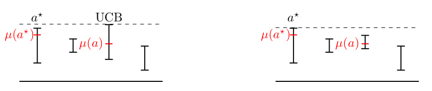
Illustration of the UCB algorithm. Left: A a suboptimal action has higher UCB than the optimal action. Right: a suboptimal action is taken and corresponding confidence interval shrink substantially.
Why regret is bounded under UCB
- $a_t = a^*$
- No regret incurred
- $a_t \not= a^*$
- If this happens, the confidence interval for $a_t$ must be quite large, due to $\mu(a_t) < \mu(a^*)$
- Even though we incur regret, the confidence interval of $a_t$ will shrink dramatically and $\hat{\mu}(a_t) \rightarrow \mu(a_t)$
- Every time we incur regret, we learn a lot about the unknown means
I am a bit confused about how $\operatorname{conf}_t(a)$ should be set. Assume the game process to round $t$, and at each around we compute $A$ confidence bounds for $A$ arms. If we want all $AT$ confidence bounds computed along the way to hold. By Hoeffding’s Inequality,
\[\begin{align} \exp \left( \frac{-2N_t(a) \varepsilon^2}{(0-1)^2} \right) &= \delta/AT \\ 2N_t(a) \varepsilon^2 &= \log(AT/\delta) \\ \varepsilon &= \sqrt{\frac{\log(AT/\delta)}{2N_t(a)}} \\ \end{align}\]This is slightly different from Krishnamurthy’s result and is also different from the UCB1 of the original UCB paper (their result is $\log(T)$ instead of $\log(AT)$, so they only update confidence bound of one arm at each step?).
Theorem Regret bound of UCB
UCB ensures that with probability $\geq 1-\delta$,
\[T\mu(a^*) - \sum_{t=1}^T \mu(a_t) \leq O(\sqrt{AT\log(AT/\delta)})\]proof
Step 1. $\mu(a^*) − \mu(a_t)$ are bounded
\[\begin{align} \mu(a^*)-\mu(a_t) &=\mu(a^*)-\hat{\mu}_{t-1}(a^*)+\hat{\mu}_{t-1}(a^*)-\hat{\mu}_{t-1}(a_t)+\hat{\mu}_{t-1}(a_t)-\mu(a_t) \\ & \leq \operatorname{conf}_{t-1}(a^*)+\hat{\mu}_{t-1}(a^*)-\hat{\mu}_{t-1}(a_t)+\operatorname{conf}_{t-1}(a_t) \\ & \leq \operatorname{conf}_{t-1}(a_t)+\hat{\mu}_{t-1}(a_t)-\hat{\mu}_{t-1}(a_t)+\operatorname{conf}_{t-1}(a_t) \\ & \leq 2 \cdot \operatorname{conf}_{t-1}(a_t) \end{align}\]The second last line is obtained by UCB procedure: \(a_t = \operatorname{argmax}_a \hat{\mu}_{t-1}(a) + \operatorname{conf}_{t-1}(a)\). Therefore, UCB of $a_t$ is no less than UCB of $a^*$.
Step 2. $\sum \mu(a^*) − \mu(a_t)$ are bounded
\[\sum_t [\mu(a^*)-\mu(a_t)] \leq 2 \sum_t \operatorname{conf}_{t-1}(a_t) \leq 4AT\sqrt{\log{2AT/\delta}}\]We will skip the algebraic manipulations in this step, interested read please refer to here.