Concentration Inequality
This post is mainly based on
The term concentration inequality originate from concentration of measure. In short, concentration of measure describes the phenomenon that the sum of independent variables, say, each with range $O(1)$, sharply concentrates in a much narrower range, e.g., $O(\sqrt{n})$ as oppose to its possible range $O(n)$. Terence Tao describes this topic in details in his blog.
Concentration inequality describes the probability of the above sum falling out of this narrower range. Concentration inequality can be used to measure the failure probability of machine learning model.
In this post, we will focus on concentration inequality, probability tools and algebraic tools that will be used in bandit problem.
Probability Tools
1. Expectations
Let $X, Y, X_i$ be random variables
Independence: $\mathbb{E}[\sum X_i] = \sum \mathbb{E}[X_i]$
Conditional Expectation: $\mathbb{E}_Y[Y |X = x] = \int y p(y|x) \mathop{}\mathrm{d}y$
Law of Total Expectation / Iterated Expectations
\[\mathbb{E}_Y[Y] = \mathbb{E}_X[\mathbb{E}_Y[Y|X]] = \int \mathbb{E}_Y[Y |X = x] p(x) \mathop{}\mathrm{d}x\]2. Variance
Variance: $\operatorname{Var}[X] = \mathbb{E}[(X - \mathbb{E}[X])^2] = \mathbb{E}[X^2] - \mathbb{E}[X]^2$
Independence: $\operatorname{Var}[ \sum a_i X_i ] = \sum a_i^2 \operatorname{Var}[X_i]$
Law of total variance
\[\operatorname{Var}[Y] = \operatorname{Var}[\mathbb{E}_Y[Y|X]] + \mathbb{E}_X[\operatorname{Var}[Y|X]]\]proof
\[\begin{align} \operatorname{Var}(Y|X) &= \mathbb{E}[Y^2|X] - \mathbb{E}[Y|X]^2 \\ \mathbb{E}_X[\operatorname{Var}(Y|X)] &= \mathbb{E}_X[\mathbb{E}_Y[Y^2|X]] - \mathbb{E}_X[\mathbb{E}[Y|X]^2] \\ \mathbb{E}[\operatorname{Var}(Y|X)] &= \mathbb{E}[Y^2] - \mathbb{E}[\mathbb{E}[Y|X]^2] \\ \mathbb{E}[\operatorname{Var}(Y|X)] &= (\mathbb{E}[Y^2] - \mathbb{E}[Y]^2) - (\mathbb{E}[\mathbb{E}[Y|X]^2] - \mathbb{E}[Y]^2)\\ \mathbb{E}[\operatorname{Var}(Y|X)] &= \operatorname{Var}(Y) - (\mathbb{E}[\mathbb{E}[Y|X]^2] - \mathbb{E}[Y]^2)\\ \operatorname{Var}(Y) &= \mathbb{E}[\operatorname{Var}(Y|X)] + \mathbb{E}_X[\mathbb{E}_Y[Y|X]^2] - (\mathbb{E}_X[\mathbb{E}_Y[Y|X]])^2\\ \operatorname{Var}(Y) &= \mathbb{E}[\operatorname{Var}(Y|X)] + \operatorname{Var}(\mathbb{E}[Y|X]) \end{align}\]Line 3 by law of total expectation. Last line by definition of variance on $\mathbb{E}_Y[Y|X]$
3. Union Bound
\[P[x \in A \cup B] ≤ P[x \in A] + P[x \in B]\]4. Moment Generating Function
\[M_X(t) = \mathbb{E}[e^{tX}]\]Moment generating function can be used to describes the tail behavior of a distribution: how likely it is that the random variable takes values far away from its expectation. For details, see Chernoff bound below.
Algebraic Tools
1. Jensen’s Inequality
For a convex function $f$,
\[f(tx_{1}+(1-t)x_{2})\leq tf(x_{1})+(1-t)f(x_{2})\]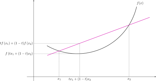
If $X$ is a random variable and $\phi$ is a convex function, then
\[\varphi (\operatorname {E} [X])\leq \operatorname {E} \left[\varphi (X)\right]\]2. Cauchy–Schwarz Inequality
For all vectors $u$, $v$ of an inner product space,
\[|\langle u, v \rangle | \leq \|u\| \|v\|\]3. AM-GM Inequality
AM stands for arithmetic mean: $\frac {x_1+x_2+\cdots +x_n}{n}$, GM stands for geometric mean: $\sqrt[{n}]{x_1 \cdot x_2 \cdots x_n}$. AM-GM Inequality is,
\[\frac {x_{1}+x_{2}+\cdots +x_{n}}{n} \geq \sqrt[ {n}]{x_{1}\cdot x_{2}\cdots x_{n}}\]For $n=2$,
\[\frac {x+y}{2}\geq \sqrt {xy}\]Markov’s Inequality
If $X$ is a random variable and $X$ is non-negative, then for any $\varepsilon > 0$
\[P[X \geq \varepsilon] \leq \frac{\mathbb{E}[X]}{\varepsilon}\]proof
\[\begin{align} P[X \geq \varepsilon] &= \int_\varepsilon^\infty p(x) \mathop{}\mathrm{d}x \\ &= \int_\varepsilon^\infty \frac{x}{x}p(x) \mathop{}\mathrm{d}x \\ &\leq \int_\varepsilon^\infty \frac{x}{\varepsilon}p(x) \mathop{}\mathrm{d}x \\ &\leq \int_0^\infty \frac{x}{\varepsilon}p(x) \mathop{}\mathrm{d}x \\ &\leq \frac{1}{\varepsilon} \mathbb{E}[X] \end{align}\]Chebyshev’s Inequality
If $X$ is a random variable with finite mean and variance, then for any $\varepsilon > 0$,
\[P(|X-\mathbb{E}[X]| \geq \varepsilon) \leq \frac{\operatorname{Var}[X]}{\varepsilon^2}\]proof
Since Markov’s inequality requires positive random variable, we can square $X-\mathbb{E}[X]$: \(\begin{align} P(|X-\mathbb{E}[X]| \geq \varepsilon) &= P((X-\mathbb{E}[X])^2 \geq \varepsilon^2) \\ &\leq \frac{\mathbb{E}[(X-\mathbb{E}[X])^2]}{\varepsilon^2} \\ &= \frac{\operatorname{Var}(X)}{\varepsilon^2} \end{align}\)
The second line is obtained by apply Markov’s inequality on $Y = (X-\mathbb{E}[X])^2$.
Sums of Independent Variables + Chebyshev’s Inequality
Consider iid random variables $X_1 , … , X_n$ with
- $\mathbb{E}[X_i] = \mu$
- $\operatorname{Var}(X_i) = \sigma^2 < \infty$.
Let $\bar{X} = \frac{1}{n} \sum X_i$. $\bar{X}$ can be viewed as an empirical estimation of $\mu$.
We are interested in how close is our estimation $\bar{X}$ to the ground truth $\mu$. Or the tail probability of $\delta = P(| \bar{X} - \mu | \geq \varepsilon)$. Concentration inequality provide bounds on how a random variable $X$ deviates from some value (e.g., $\mathbb{E}[X]$).
The above tail probability can be estimated by Chebyshev’s inequality. Since variance of $\bar{X}$ is $\sigma^2/n$, we have
\[P(| \bar{X} - \mu | \geq \varepsilon) \leq \frac{\sigma^2}{n\varepsilon^2}\]Since we are interested in the tail probability $\delta$, let $\frac{\sigma^2}{n\varepsilon^2} = \delta$ and solve for $\varepsilon$, we have
\[\varepsilon = \sqrt{\frac{\sigma^2}{n\delta}}\]Therefore, with probability $1-\delta$, we have $P(| \bar{X} - \mu | \leq \sqrt{\frac{\sigma^2}{n\delta}}) $. Or we are confident that our estimation is $\sqrt{\frac{\sigma^2}{n\delta}}$ close to the true mean.
- When $n$ increase (more samples), the error bound becomes tighter
- Error bound converge at a $\sqrt{1/n}$ rate, as predicted by the central limit theorem
- When $1-\delta$ increase (higher confidence in our estimation), the error bound becomes looser
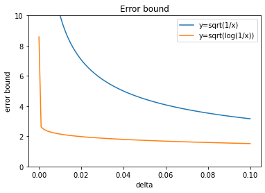
- Error bound converge at a $\sqrt{1/\delta}$ rate, which is quite bad. This reason is we will to take a union bound $k$ events of this type. Therefore, the failure probability required for each event is $\delta/k$ and this could make the error bound quite high (see plot in next section).
Chernoff bound
If we have information about higher moments, it is better to apply Markov’s inequality to $e^{tX}$ and get the moment generating function:
\[P(X \geq \varepsilon)=P(e^{tX}\geq e^{t\varepsilon}) \leq \frac{\mathbb{E}[e^{tX}]}{e^{t\varepsilon}} = M_X(t)\exp(-t\varepsilon)\]Since this bound is true for every $t$, we have:
\[P(X \geq \varepsilon) \leq \inf_{t \geq 0} M_X(t)\exp(-t\varepsilon)\]If we have more information about the distribution, we can just substitute the moment generating function. For example, $X \sim N(0, 1)$ and $M_X(t) = \exp(t^2/2)$
\[P(X \geq \varepsilon) \leq \inf_{t \geq 0} \exp(t^2/2 -t\varepsilon) = \exp(-\varepsilon^2/2)\]Solve for $\delta = \exp(-\varepsilon^2/2)$, we have $\varepsilon = \sqrt{2\log \frac{1}{\delta}}$. By adding information on distribution, the Chernoff bounds yields a tighter error bound $O(\sqrt{\log \frac{1}{\delta}})$ than the error bound of Chebyshev’s inequality $O(\sqrt{\frac{1}{\delta}})$.
Hoeffding’s Inequality
Chernoff bounds requires information of the distribution which could be unavailable in practice. Hoeffding’s inequality relax this condition by only requiring the random variable to be bounded in $[a,b]$ almost surely. We will skip the proof since it requires Hoeffding’s lemma which is a bit technical.
Let $X_1, …, X_n$ by iid random variables with mean $\mu$ such that $a_i \leq X \leq b_i$ almost surely for all $i$. Then with $\bar{X} = \frac{1}{n} \sum X_i$, we have,
\[P(\bar{X} - \mu \geq \varepsilon) \leq \exp\left( \frac{-2n^2\varepsilon^2}{ \sum (a_i-b_i)^2 } \right)\]If all $X_i$ have same bound $[a,b]$ and using symmetry,
\[P( | \bar{X} - \mu | \geq \varepsilon) \leq 2\exp\left( \frac{-2n\varepsilon^2}{(a-b)^2 } \right)\]Solving for $\delta = 2\exp\left( \frac{-2n\varepsilon^2}{(a-b)^2 } \right) $, we have $\varepsilon = \sqrt{ \frac{(a-b)^2}{2n}\log \frac{2}{\delta}}$.
Bernstein Inequality
Hoeffding’s inequality only use the information that $X_i$ is bounded. If the variance of $X_i$ is small, we can obtain a sharper error bound using Bernstein’s inequality. The proof is too technical so we will just state the result:
Let $X_1, …, X_n$ by iid random variables with mean $0$ such that $| X | \leq M$ for all $i$,
\[P(\sum X_i \geq \varepsilon) \leq \exp \left( -\frac{\varepsilon^2/2}{\sum \mathbb{E}[X_i^2] + M\varepsilon/3} \right)\]Let $\bar{X} = \frac{1}{n} \sum X_i$ and solve for $\varepsilon$, we have,
\[|\bar{X}| \leq \sqrt{\frac{2\mathbb{E}[X_i^2]\log(2/\delta)}{n}} + \frac{2M \log(2/\delta)}{3n}\]When $\operatorname{Var}(X) \ll M$, Bernstein inequality provides a tighter error bound than Hoeffding’s inequality. For example, let $\operatorname{Var}(X)=1, M=10, n=100$, Bernstein inequality’s error bound is $\sqrt{1/50\log(2/\delta)} + 1/15\log(2/\delta) $ while Hoeffding’s inequality’s error bound is $\sqrt{2\log(2/\delta)}$.