Time Series Precision Recall
This post is mainly based on
Time Series Prediction
Time series (TS) predictions are often modelled as regression problems. However, in many scenarios,
- Minimizing MSE may not be the correct optimization goal
- We may not need a continuous forecast of future
MSE as optimization goal
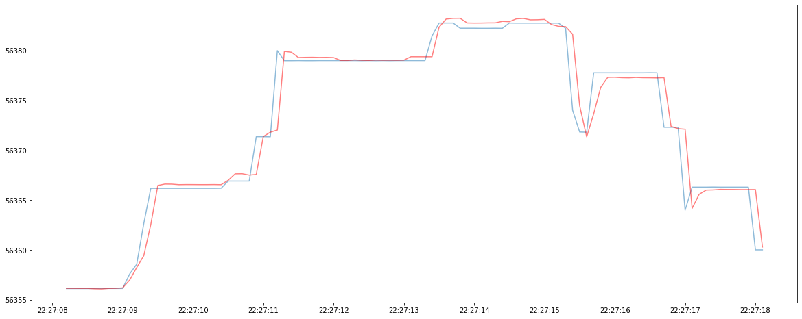
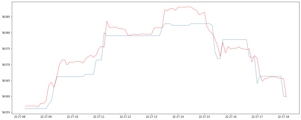
To illustrate why minimizing MSE may not be the correct optimization goal, consider the two TS forecasting models below: the blue line represent the ground truth TS and the red line represent the continuous forecasted TS. Although Model 1 has a lower MSE, it produce virtually useless forecast since the predicted TS always lag behind the ground truth TS. In comparison, Model 2 has a higher MSE, but it could be useful since its prediction leads the ground truth TS in many cases.
TS Model 1:
TS Model 2:
Continuous forecast
Many TS modelling problems can be viewed as anomaly detection. Consider the early detection of the acute kidney injury (AKI) in ICU. What we are interested in, is forecasting the future jump in creatinine level, instead of a continuous prediction across all time steps.
We will consider modelling TS as anomaly detection problems in this post. Given a classification model (for each time step, the model predicts anomaly vs normal), the standard evaluation metric is Precision and Recall:
\[\text{Precision} = \frac{TP}{TP + FP}\] \[\text{Recall} = \frac{TP}{TP + FN}\]Precision and recall is designed to evaluate independently drawn point-based data. However, most of the real world anomaly detection problems are range based. Suppose the AKI prediction model yield the following result:
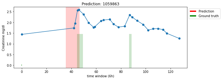
The shaded red region represent predicted anomaly; the shaded green region represent ground truth anomaly.
A qualitative description:
- The model correctly predict the first anomaly, but the prediction only overlap with the front end of the ground truth
- The model missed the second anomaly
For another time series:
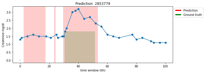
A qualitative description:
- The model falsely predict the first and the second anomaly
- The model correctly predict the third anomaly, but the prediction range is too wide
However, a quantitatively evaluation could be complex. We need to consider:
- How to evaluate partial overlaps
- A single prediction range could be partially TP and FP at the same time
- The position of the overlap could be important
- For detection problem, overlapping with the front end of the ground truth range is more important
- If each ground truth anomaly is detected as a single unit or not
- For certain use cases, detecting one ground truth range as segmented prediction is problematic
Precision and Recall for Time Series
The Precision and Recall for Time Series (PRTS) metric is proposed with the following goals:
- Expressive: captures criteria unique to range-based anomalies, e.g., overlap position and cardinality.
- Flexible: supports adjustable weights across multiple criteria for domain-specific needs.
- Extensible: supports inclusion of additional domain-specific criteria that cannot be known a priori.
Notations
- $R, R_i$: set of ground truth / real anomaly ranges, the $i$-th real anomaly range
- $P, P_j$: set of predicted anomaly ranges, the $j$-th predicted anomaly range
- $N , N_r , N_p$: number of all points, number of real anomaly ranges, number of predicted anomaly ranges
- $\alpha$ relative weight of existence reward
- $\gamma()$: overlap cardinality function
- $\omega()$: overlap size function
- $\delta()$: positional bias function
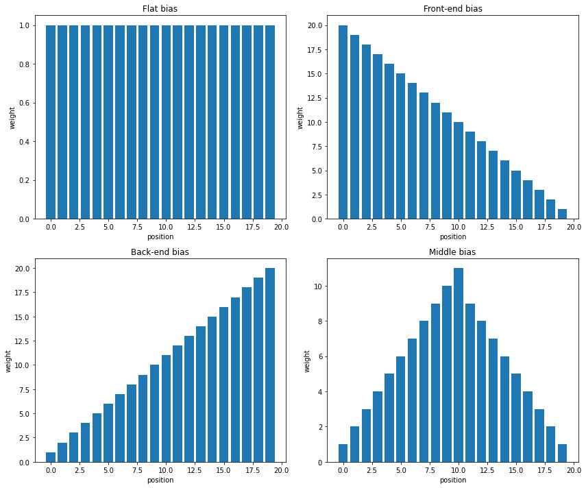
Positional Bias
Positional bias measures relative importance prediction based on its position. The positional bias function $\delta$ takes position $i$, range length and output weight:
def delta(i, range_length):
    \\ calculations
    return weight
Below are visualizations of 4 positional bias of defined by the paper:
Existence Reward
Existence reward is a part of the recall calculation. The goal is to measure the detection of ground truth $R_i$. It produce a binary output and overlapping is not considered.
\[\text{Existence Reward}(R_i, P) = \left\{\begin{array}{l} 1, \text { if } \sum_{j=1}^{N_p} |R_i \cap P_j| \geq 1 \\ 0, \text { otherwise } \end{array}\right.\]Overlap Cardinality
The goal of overlap cardinality is to penalize fragmentation
- For recall, it penalize fragmented prediction $P_1, P_2, …$ on one ground truth $R_i$
- For precision, it penalize predicting one range $P_i$ to cover multiple ground truth $R_1, R_2, …$
For recall, the overlap cardinality is defined as:
\[\text{Cardinality Factor}(R_i, P) = \left\{\begin{array}{l} 1, \text{ if } R_i \text{ overlaps with at most one } P_j \in P\\ \gamma(R_i, P), \text{ otherwise} \end{array}\right.\]Let $x$ be the number of distinct prediction overlap with ground truth range $R_i$. Since the goal is to penalize if model generate many predictions for one ground truth range, we can choose $\gamma = 1/x$.
For precision, the overlap cardinality is defined as:
\[\text{Cardinality Factor}(P_i, R) = \left\{\begin{array}{l} 1, \text{ if } P_i \text{ overlaps with at most one } R_j \in R\\ \gamma(P_i, R), \text{ otherwise} \end{array}\right.\]Overlap Reward
Overlap size function $\omega$ measures the overlap between ground truth range and predicted range.
def omega(gt_range, overlap_range, delta):
    value = 0
    value_max = 0
    gt_length = len(gt_range)
    for i in range(0, gt_length):
        bias = delta(i, gt_length)
        value_max = value_max + bias
        if gt_range[i] in overlap_range:
            value = value + bias
    return value/value_max
$\omega$ is defined differently for precision and recall:
- Recall: $\omega(R_i, R_i \cap P_j , \delta)$
- Precision: $\omega(P_i, P_i \cap R_j , \delta)$
For recall, Overlap Reward is defined as sum of Overlap Size over $R_i$, penalized by Cardinality Factor:
\[\text{Overlap Reward}(R_i, P) = \text{Cardinality Factor}(R_i, P) \times \sum_{j=1}^{N_p} \omega(R_i, R_i \cap P_j , \delta)\]For precision,
\[\text{Overlap Reward}(P_i, R) = \text{Cardinality Factor}(P_i, R) \times \sum_{j=1}^{N_r} \omega(P_i, P_i \cap R_j , \delta)\]Range-based Recall
The overall Range-based Recall $\text{Recall}_T(R,P)$ is defined as the mean of individual recalls:
\[\text{Recall}_T(R,P) = \frac{1}{N_r} \sum_{i=1}^{N_r} \text{Recall}_T(R_i,P)\]Individual recall is defined as a weight sum between Existence Reward and Overlap Reward:
\[\text{Recall}_T(R_i,P) = \alpha \cdot \text{Existence Reward}(R_i, P) + (1-\alpha) \cdot \text{Overlap Reward}(R_i, P)\]where the relative weight is controlled by hyperparameter $\alpha$.
Range-based Precision
The overall Range-based Precision $\text{Precision}_T(R,P)$ is defined as the mean of individual precisions:
\[\text{Precision}_T(R,P) = \frac{1}{N_p} \sum_{i=1}^{N_p} \text{Precision}_T(P_i, R)\]Individual precision just consider Overlap Reward:
\[\text{Precision}_T(P_i, R) = \text{Overlap Reward}(P_i, R)\]Discussion
I find this paper interesting, due to:
- The valuation metric is tunable and can be customized to individual problem
- The idea of Positional Bias and Cardinality Factor is useful when considering what is important to our application
- Positional Bias and Cardinality Factor can be easily implemented into loss function to encourage certain behavior of the model