ROC and PR Curve

ROC curve, PR Curve and area under curve (AUC) are often used for classification model comparison in the machine learning.

Problem setup

For simplicity, consider a binary classification problem modelled by Logistic regression,

\[p(x)=\frac {1}{1+e^{-\beta x}}\]

The model maps $x$ to a real value $p(x)$. To fit the model, we could perform a MLE optimization to find its parameter $\beta$:

\[\text{argmax}_{\beta} \Pr(Y|X;\beta) = \text{argmax}_{\beta} \prod_i p(x_i;\beta)^{y_i} (1-p(x_i;\beta))^{1-y_i} = \text{argmax}_{\beta} \prod_i \frac{e^{\beta x_i y_i}}{1+e^{\beta x_i}}\]

A threshold is required to make a prediction: if $p(x_i;\beta) > \text{threshold}$, the model output positive. The default threshold is $0.5$. We can change the aggressiveness of the model by adjusting the decision boundary (say, predict positive when $p(x) > 0.4$).

Confusion matrix

Confusion matrix is a table specifies 4 types of outcomes of a binary prediction. The term “Positive” and “Negative” represents predicted outcome and the term “True” and “False” represents the correctness of predicted outcome.

Outcomes	Predict Positive	Predict Negative
Ground Truth Positive	True Positive (TP)	False Negative (FN)
Ground Truth Negative	False Positive (FP)	True Negative (TN)

When we change the decision threshold, the confusion matrix will change.

Sensitivity and specificity

According to wikipedia, the terms “sensitivity” and “specificity” were introduced by American biostatistician Jacob Yerushalmy in 1947. It has strong connections to medical field and clinical trails.

\[\text{Sensitivity} = \frac{TP}{TP + FN} = \Pr(\hat{Y}=1 | Y=1)\] \[\text{Specificity} = \frac{TN}{TN + FP} = \Pr(\hat{Y}=0 | Y=0)\]

If we lower the threshold, the model will be more aggressive in predicting positive labels. Therefore, $\Pr(\hat{Y}=1 \cap Y=1)$ will increase, while $\Pr(Y=1)$ remains unchanged. Sensitivity will increase $\Pr(\hat{Y}=1 | Y=1)$. By similar arguments, specificity will decrease. Changing threshold can be viewed as a trade-off between sensitivity and specificity.

Depending on the nature of the prediction task, we may focus on a higher sensitivity or specificity. Consider a diagnosis test for cancer where the patient will go through a surgery if the test returns positive. We cannot afford making mistakes to cause suffering of a patient, therefore the model should have high specificity. Alternatively, consider a screening test for a rare disease where patients will go through further tests for diagnosis. In this case, the cost for missing a patient is high, therefore the model should have high sensitivity.

ROC curve

ROC curve strands for receiver operating characteristic curve. As previously mentioned, there is usually a trade-off between sensitivity and specificity at different threshold. ROC curve is a method for visualizing sensitivity and specificity at all threshold levels. It is commonly used to compare model performance in machine learning.

Some notations,

\[\text{FP-rate} = \frac{FP}{TN + FP} = 1-\text{Specificity} = \Pr(\hat{Y}=1 | Y=0)\] \[\text{TP-rate} = \text{Sensitivity} = \Pr(\hat{Y}=1 | Y=1)\]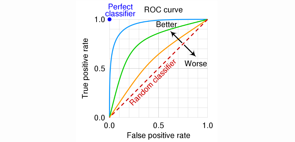

For ROC curve, the x-axis is FP-rate; the y-axis is TP-rate. Area under curve (AUC) can be used as a quantitative metric to compare two models. For a random model, both $\Pr(\hat{Y}=1 | Y=0)$ and $\Pr(\hat{Y}=1 | Y=1)$ equal to the threshold value. Therefore, the plot is a diagonal and AUC is 0.5. For a “good” model, given a specificity level, the sensitivity will be higher. Therefore, points on the ROC curve: $(1-\text{Specificity}, \text{Sensitivity})$, will be closer to the point $(0,1)$, resulting in a higher AUC.

ROC space

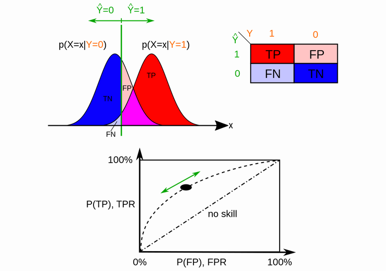
In next step, we will put ROC curve into a probabilistic framework. Let $X = p(x)$, where $p(x)$ is the function which maps an example to a real value (a score). Recall that $x$ are examples sampled from some generator function. Then $X$ will be a random variable. We will split $x$ into 2 groups: $x$ sampled from ground truth positive label ($Y=1$) and ground truth negative label ($Y=0$). Then, $X|Y=1$ and $X|Y=0$ will induce 2 distribution. Let $f_1$ and $f_0$ be their density function and $T$ be the threshold. We have,

\[\text{TP-rate}(T) = \int_T^\infty f_1(x)\,dx\] \[\text{FP-rate}(T) = \int_T^\infty f_0(x)\,dx\]

Evaluating the above integral for different T will produce the ROC curve. The ROC space is induced by all possible mappings $p(x)$. In practice, we don’t know $f_1$ and $f_0$, but they can be approximated by from samples (i.e., training or testing data).

For implementation, Given y_true and y_score, we can compute a rank of positive predicting. Using this rank, we can essentially asked the question: if the threshold is increased by one rank, how does the confusion matrix change. It can be shown that the ROC AUC is closely related to the Mann–Whitney U test and Wilcoxon test of ranks. If you are interested in this topic, you can read more here.

ROC AUC also face some criticism

• Small-sample precision of ROC-related estimates
• AUC: a misleading measure of the performance of predictive distribution models

PR curve

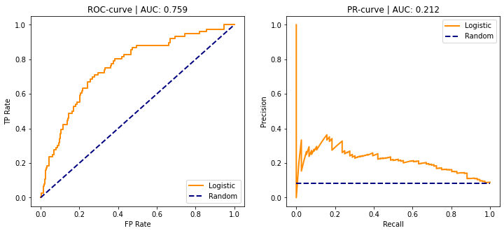
PR curve stands for precision recall curve. It is another method for visualizing model performance. Model is evaluated by its precision and recall at different threshold levels.

\[\text{Precision} = \frac{TP}{TP + FP} = \Pr(Y=1 | \hat{Y}=1)\] \[\text{Recall} = \text{Sensitivity} = \Pr(\hat{Y}=1 | Y=1)\]

For PR curve, the x-axis is Recall; the y-axis is Precision. Assume we have a predictive model. For a random model, the precision will be $\Pr(Y=1)$ regardless of recall and AUC is $\Pr(Y=1)$. As the threshold decrease, the model will be more aggressive in predicting positive. Recall will increase, and precision is likely decreased, resulting in a downward trend in PR-curve. Unlike ROC curve, PR curve is non-convex. The reason is that there is no guarantee that the model have higher precision at say, 0.9 recall level than 0.8 recall level.

Imbalanced data

Most practitioner believes that PR-curve should be preferred on imbalanced dataset / rare event detection. The reason is as follow: assume that rare event are labeled as positive or $Y=1$, then

ROC Curve measures 1 metric on positive class and 1 metric on negative class:

• Sensitivity = $\Pr(\hat{Y}=1 | Y=1)$
• 1-Specificity = $\Pr(\hat{Y}=1 | Y=0)$

PR Curve measures 2 metrics on positive class

• Precision = $\Pr(Y=1 | \hat{Y}=1)$
• Recall = $\Pr(\hat{Y}=1 | Y=1)$

In rare event detection, we only care about performance on positive class, which is adequately measured by PR Curve. In comparison, ROC curve measures something about negative class: $ \Pr(\hat{Y}=1 | Y=0) $, which is not really useful since most samples are negative and any decent model should output very low $\Pr(\hat{Y}=1 | Y=0)$. One can image 2 models where Model A has very high precision $\Pr(Y=1 | \hat{Y}=1)$ and Model B has lower precision. In context of rare event detection, model-A should clearly be preferred. However, the difference between A and B on ROC curve could be very small, we will use an example to illustrate this:

Consider a dataset with 1 million examples and 100 positive labels. There are two models:

• Model A: TP = 90, FP = 10, FN = 10, TN ~= 1e6
• Model B: TP = 90, FP = 1910, FN = 10, TN ~= 1e6

Suppose we have only the above single point on ROC and PR curve

ROC curve:

• Model A
  • $\text{FP-rate} = 10/(10^6-100) = 0.00001$
  • $\text{TP-rate} = 90/100 = 0.9$
• Model B:
  • $\text{FP-rate} = 1910/(10^6-100) = 0.00191$
  • $\text{TP-rate} = 90/100 = 0.9$

PR curve:

• Model A:
  • $\text{Precision} = 90/100 = 0.9$
  • $\text{Recall} = 90/100 = 0.9$
• Model B:
  • $\text{Precision} = 90/2000 = 0.045$
  • $\text{Recall} = 90/100 = 0.9$

Due to TP = 90 for both model, the Recall is the same. On ROC curve, the difference in FP-rate is 0.0019, resulting in a very small difference in ROC AUC. However, on PR curve, the difference in Precision is 0.855 and the difference in PR AUC is large. Original discussion can be found here and here.

Note that the above analysis is based on the assumption that both models have very high precision. For Model A, $\Pr(Y=1 | \hat{Y}=1) = 0.9$. For Model B, $\Pr(Y=1 | \hat{Y}=1) = 0.045$. You may think precision of Model B is low, however, when comparing to a random model ($\Pr(Y=1 | \hat{Y}=1) = 0.0001$), Model B implies a 450x improvement in precision (Model A implies a 9000x improvement).

Recall that the FP-rate is computed as $\frac{FP}{TN + FP}$. A high precision model result in a negligible numerator compared to denominator (10 or 1910 $\ll 10^6$). The reason why ROC is bad, is that FP-rate is insensitive to change in FP relative to a very big negative class in denominator, resulting in Model A only show very small advantage over model B. However, for a low precision model, say, Model A and B have 2x vs 10x improvement in precision. Then, their FP-ratio difference will be approximately $0.45 - 0.09 = 0.36$, which is more significant.

In context of rare event detection, a “useful” model is required to have high precision. Therefore, PR curve should be preferred in model evaluation.

ROC space vs PR space

One might be interested in the relationship between ROC space and PR space. For example, is optimizing for ROC AUC and PR AUC equivalent? Below is a summary of 3 interesting results from this paper. More discussions here.

One-to-one mapping

ROC curve $\Longleftrightarrow$ PR curve, due to each point on ROC curve corresponds to a unique point on PR curve. Proof is trivial, one point on ROC-curve $\Longleftrightarrow$ a unique confusion matrix $\Longleftrightarrow$ one point on PR curve.

ROC/PR dominance

Curve I dominate Curve II in ROC space $\Longleftrightarrow$ Curve I dominate Curve II in PR space

The idea is to use proof by contradiction: given curve I dominate curve II in ROC space, assume there is a pair of point on the corresponding PR curve where: Precision of point on curve II > Precision of point on curve I, given same recall. We can show this is impossible. The proof is a bit tedious and readers can refer to the paper for details.

ROC/PR non-dominance

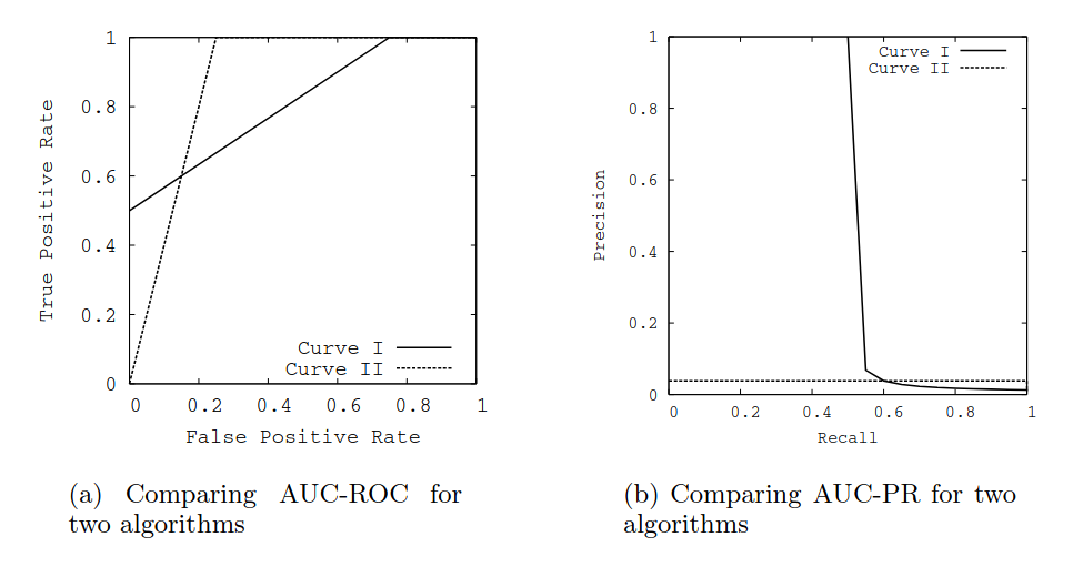
If there is no dominance relationship between two curves in ROC/PR space. Then a higher ROC AUC does not implies a higher PR AUC and vice versa. Below is an example from there paper where authors plays with the rank of the half of the positive examples. In this example Curve II has higher ROC AUC, but Curve I has higher PR AUC:

• ROC AUC
  • Curve I: 0.813
  • Curve II: 0.875
• PR AUC
  • Curve I: 0.514
  • Curve II: 0.038

$F_\beta$ score

Precision and recall are complementary and $F_\beta$ score is a measure that combines precision and recall,

\[F_\beta = (1+\beta^2)\frac{\text{precision} \cdot \text{recall}}{\beta^2 \cdot \text{precision} + \text{recall}} = \frac{1}{\frac{\beta^2}{1+\beta^2} \frac{1}{\text{recall}} + \frac{1}{1+\beta^2} \frac{1}{\text{precision}}}\]

where the parameter $\beta$ controls the relative importance of recall to precision. For a high $\beta$, the recall dominate the $F_\beta$ score.

The $F_1$ score is the harmonic mean between precision and recall,

\[F_1 = 2\frac{\text{precision} \cdot \text{recall}}{\text{precision} + \text{recall}} = \frac{2}{1/\text{precision} + 1/\text{recall}}\]