Recurrent Neural Network
This post is mainly based on
- Advances in Optimizing Recurrent Networks, IEEE 2013
- On the difficulty of training recurrent neural networks, PMLR 2013
- Empirical Evaluation of Gated Recurrent Neural Networks on Sequence Modeling, 2014
- An Empirical Exploration of Recurrent Network Architectures, PMLR 2015
- LSTM: A Search Space Odyssey, IEEE 2016
RNN
A RNN is an autoregressive model: a model which predict a future outcome based on previously observed outcomes:
\[h_t = F_\theta(h_{t−1}, x_t)\]where $x_t$ is the input at time $t$ and $h_t$ is the hidden state at time $t$. A reasonable choice of $F_\theta$ could a composition of a $\tanh$ activation and a fully connected layer:
\[h_t = \tanh(W_x x_t + W_h h_{t-1} + b)\]where $W_x, W_h$ are weight matrices for input and previous state and $b$ is bias. We can also stack multiple hidden layers on top of each other, resulting in a Multi-layer RNN.
\[h_{k,t} = \tanh(W_{k,x} h_{k-1, t} + W_{k,h} h_{k,t-1} + b)\]where $k$ is the number of layer, $h_{0, t} = x_t$.
One of the main goals of CNN is to learn a good representation from visual inputs, where weights of the Conv filters are shared across different positions; similar argument can be applied to RNN: when we unfolded a RNN computation through time, we can clearly sees a deep neural network with shared weights across time.
Backpropagation Through Time (BPTT)
Automatic differentiation on a RNN computation graph involves calculating products of Jacobians on $h_t$, which naturally leads to exploding or vanishing gradient problem. Consider taking gradient on a RNN from $t_1$ to $t_2$:
\[\frac{ \partial h_{t_2}}{ \partial h_{t_1} } = \prod_{t = t_{1+1}}^{t_2} \frac{ \partial h_t}{ \partial h_{t-1} }\]Assume $t_2 - t_1$ is large, when the dominate eigenvalue of $\frac{ \partial h_t}{ \partial h_{t-1} } > 1$, $\frac{ \partial h_{t_2}}{ \partial h_{t_1} }$ will explode; when the dominate eigenvalue of $\frac{ \partial h_t}{ \partial h_{t-1} } < 1$, $\frac{ \partial h_{t_2}}{ \partial h_{t_1} }$ will vanish. Therefore, gradient on $\theta$ is pretty unstable:
\[\frac{\partial L(y, \hat{y}_{t_2})}{\partial \theta} = \sum_{t = t_1}^{t_2-1} \frac{\partial L(y, \hat{y}_{t_2})}{\partial h_{t_2}} \frac{ \partial h_{t_2}}{ \partial h_{t} } \frac{ \partial h_{t}}{ \partial \theta }\]Detailed discussions can be found at Section 2 of the 2013 paper.
Section 2 of the 2015 paper, further elaborate the crux of the vanishing gradient problem: The vanishing gradient is more challenging because it does not cause the gradient itself to be small; while the gradient’s component in directions that correspond to long-term dependencies is small, the gradient’s component in directions that correspond to short-term dependencies is large. As a result, RNNs can easily learn the short-term but not the long-term dependencies.
Mitigation
Common regularization techniques like L1 or L2 penalty on $W_h$ are considered bad ideas. Although they can prevent exploding gradients, such regularization will bias $W_h$ to zero, which restrict information pass between hidden states. This results in long term memory dampening exponentially fast. The 2013 paper also discussed a widen range of other techniques, such as clipping and regularization to bias $\frac{ \partial h_t}{ \partial h_{t-1} }$ to 1. However, due to these techniques are not widely used/implemented in practice and offer limited performance boost, we will not discuss them in this post.
LSTM & GRU
In previous section, we explained why optimizing RNN is challenging and some mitigation to fix exploding and vanishing gradient. Researchers working on these directions generally focused on optimization problem itself. Other researchers take a different approach: designing a more sophisticated $F_\theta(h_{t-1}, x_t)$ for a more stable optimization. I think some parallel can be drawn between this approach and ResNet: the latter achieve significant gain in performance due to the skip connection leads to a smoother optimization landscape as discussed in this post. (Although I don’t have any proof of LSTM or GRU also lead to a smoother optimization landscape)
Long short-term memory (LSTM) was proposed by Hochreiter and Schmidhuber in 1997 (link to the original paper). LSTM was practically ignored for more than a decade until researchers showing that it can achieve state of art performance on various of seq-2-seq modelling tasks, such as speech recognition and machine translation.
Gated recurrent unit (GRU) was proposed by Cho et al. in 2014 to simplify to computation (link to the original paper).
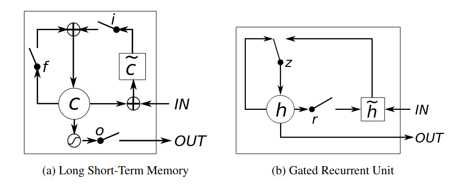 The computation graphs for LSTM and GRU are from this paper. I chose their graph over another widely referenced blog, since I believe their graphs better reflect the information flow within the recurrent units.
LSTM
Computations for LSTM are (using notations from pytorch implementation):
\[\begin{align} \begin{bmatrix} i_t \\ f_t \\ o_t \\ g_t \end{bmatrix} &= \begin{bmatrix} \sigma \\ \sigma \\ \sigma \\ \tanh \end{bmatrix} \left( W \begin{bmatrix} x_t \\ h_{t-1} \end{bmatrix} + b \right) \\ c_t &= f_t \odot c_{t-1} + i_t \odot g_t\\ h_t &= o_t \odot \tanh( c_t ) \end{align}\]Notations
- $\odot$ is Hadamard product / element-wise vector product
- $\tilde{c} = g_t$
- $f, i, o$ are forget, input, and output gates; they all use sigmoid activation and always couple with Hadamard product since their propose is to control the amount the information in range $[0,1]$ to pass through
- $g$ gate and $h_t$ use $\tanh$ activation, since their propose is to determine how to process information in range $[-1, 1]$
- The graph for LSTM has a minor error: $\tilde{c}$ doesn’t take input from $c_{t-1}$; it take input from $h_{t-1}$
GRU
Computations for GRU are (using notations from pytorch implementation):
\[\begin{align} \begin{bmatrix} r_t \\ z_t \end{bmatrix} &= \begin{bmatrix} \sigma \\ \sigma \end{bmatrix} \left( W \begin{bmatrix} x_t \\ h_{t-1} \end{bmatrix} + b \right) \\ n_t &= \tanh \left( W \begin{bmatrix} x_t \\ r_t \odot h_{t-1} \end{bmatrix} + b \right)\\ h_t &= (1-z_t) \odot n_t + z_t \odot h_{t-1}\\ \end{align}\]Notations
- $\odot$ is Hadamard product / element-wise vector product
- $\tilde{h} = n_t$
- $r, z$ are reset and update gates; they all use sigmoid activation and always couple with Hadamard product since their propose is to control the amount the information in range $[0,1]$ to pass through
- $n_t$ use $\tanh$ activation, since its propose is to determine how to process information in range $[-1, 1]$
For the computations above, weight matrices $W$ and bias vectors $b$ are not shared across different gates (I omit the subscript for gate name for simplicity).
Their experiments show that LSTM and GRU clearly outperforms vanilla RNN.
Discussions
Compared to vanilla RNN, the most prominent feature of memory update step of LSTM and GRU:
- RNN: $h_t = \tanh(W_x x_t + W_h h_{t-1} + b)$
- LSTM: $c_t = f_t \odot c_{t-1} + i_t \odot g_t$
- GRU: $h_t = (1-z_t) \odot n_t + z_t \odot h_{t-1}$
Note that both LSTM and GRU uses addition operation to update memory state, while RNN uses matrix multiplication and activation function. Multiple papers pointed out the addition operation is similar to the skip connection in ResNet: instead of computing $h_t$ directly from $h_{t-1}$, the LSTM and GRU compute $h_t$ as $\delta h_t$, where information in the old state is filtered by the $f_t$ or $z_t$.
Neural Architecture Search, 2015
LSTM and GRU are based on ad-hoc design. The motivation for the 2015 neural architecture search (NAS) paper is to determine if LSTM or GRU are optimal. The author evaluated over 10,000 different RNN architectures to check if much better architectures exist. Conclusion: they were unable to find an architecture that consistently outperforms LSTM or GRU in all experiments; they recommend to increase the bias to the forget gate before attempting to use more sophisticated approaches.
We will not go into the details of the how the NAS is conducted (e.g., what experiments are used; how to enumerate new architecture; how to tune hyperparameter). Instead, we list some of their findings:
- GRU outperformed the original LSTM on most tasks
- Adding a bias of 1 to the LSTM’s forget gate close the gap between the LSTM and GRU
- LSTM significantly outperformed all other architectures on PTB language modelling when dropout was allowed
- Forget gate is extremely important
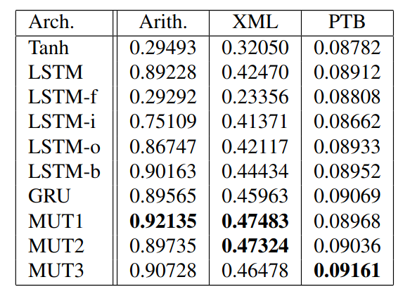
Best next-step-prediction accuracies achieved by the various architectures. LSTM-{f,i,o} refers to the LSTM without the forget, input, and output gates, respectively. LSTM-b refers to the LSTM with the additional bias to the forget gate.
While MUT1 architecture achieved better performance on accuracy, LSTM based architecture has the best performance in Negative Log Likelihood on the music datasets and Perplexities on the PTB.
Forget Gates Bias
The authors found that initializing the bias of LSTM’s forget gate to 1 results in better performance. The reason is that a random initialization effectively sets the forget gate to 0.5, which introduce a vanishing gradient with a factor of 0.5 per timestep. This problem is addressed by simply initializing the forge gates $b_f$ to a large value such as 1 or 2. By doing so, the forget gate will be initialized to a value that is close to 1, enabling better gradient flow.
Ablation Study, 2016
This 2016 paper evaluated 8 LSTM variants on 3 more realistic datasets: speech recognition (TIMIT), handwriting recognition (IAM Online), and polyphonic music modeling (JSB Chorales). In comparison, the experiments in the 2015 NAS search paper are more like synthetic benchmark (just my own opinion). They also study the importance of different hyperparameters in LSTM training. Their conclusions are:
- None of the eight investigated LSTM modifications significantly improves performance across all tasks
- Certain modifications such as coupling the input and forget gates (CIFG) or removing peephole connections (NP) simplified LSTMs without significantly decreasing performance
- Forget gate and output activation function are the most critical components of the LSTM
- Learning rate is the most crucial hyperparameter, followed by the network size
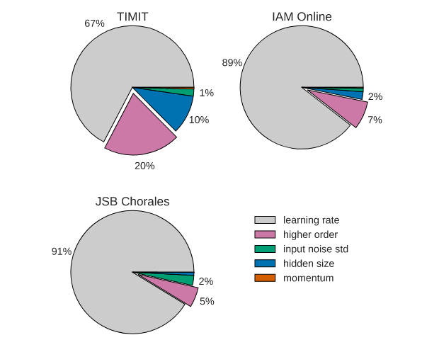
Pie charts showing which fraction of variance of the test set performance can be attributed to each of the hyperparameters. The percentage of variance that is due to interactions between multiple parameters is indicated as “higher order.”