Forward-Forward Algorithm
This post is mainly based on
- The Forward-Forward Algorithm: Some Preliminary Investigations
- Seminar: Geoff Hinton explains the Forward-Forward Algorithm
- Two implementations of supervised algorithm described in Section 3.3 of the paper
- Additional Reading: Forward Learning
This paper proposed a new learning framework:
- Replace the forward-backward pass (backpropagation) by forward-forward pass
- More aligned with how brain functions
- Show promising result on toy problems (MNIST, CIFAR-10), but are not likely to replace the existing “forward-backward” framework
Problems with Backpropagation
The paper take the stance to criticize backpropagation mainly due to:
- There is a lot of evidence suggesting that brain does not function like backpropagation
- Backpropagation requires frequent “time-outs” to perform the backward pass, which is incompatible with streaming type data
- Backpropagation requires the computation graph to be fully differentiable (No blackbox)
Why brain is not likely to implement the Backpropagation framework? Recall that Backpropagation adjusts the weight of parameters to minimize loss. The knowledge of how the weights should be adjusted is obtained in the backward pass where gradient is compute at each parameter by Automatic Differentiation. This results in inconsistency compared to how the brain functions:
- The brain needs to has perfect knowledge of computation graph (e.g., store neural activity levels), such that it can back trace the graph and compute gradient
- The brain needs to biologically know how to compute gradients for the activation function it used
There is no evidence that the brain pause to conduct a backward pass or it store neural activities. Instead, the brain functions in loops where neural activities goes through about half a dozen cortical layers in the two areas before arriving back where it started.
Forward-Forward Algorithm
Denote the two forward pass as Forward-1, Forward-2.
Key differences between the two forward passes are:
- Forward-1
- Positive data / Real data
- Expect higher layer activation
- Loss: negative sum of square of activations
- $ L(f) = -\sum_j y_{j}^2 $, where $y_j$ is output of neurons
- Minimizing loss will adjust weights to increase activations
- Forward-2
- Negative data / Fake data / Counter examples
- Expect lower layer activation
- Loss: sum of square of activations
- $ L(f) = \sum_j y_{j}^2 $, where $y_j$ is output of neurons
- Minimizing loss will adjust weights to reduce activations
Key differences between Forward-Forward Algorithm and Backpropagation are:
- Loss function
- Backpropagation: normally on computed from predict label and ground truth label
- FF algorithm: maximize/minimize the activation on each layer
- Learning goal
- Backpropagation: output the correct label
- FF algorithm: distinguish between the real and fake data on each layer
Given input data $x$, the probability of $x$ being a positive/real example estimated by layer $i$ is:
\[p(x\text{ is positive}) = \sigma(\sum_{j} y_j^2 - \theta)\]where $\theta$ is some threshold.
Key Architecture Design
- Layer normalization
- Activation is normalized to ensure activation information from previous layer is not leaked
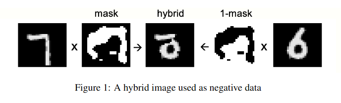
- Negative data
- Supplied / Engineered: see Figure 1 below, negative data in MNIST is a combination of 2 digits
- Generated: used the underlying network generate negative data (generative model)
- Supervise Learning
- Forward-Forward Algorithm is unsupervised / representation learning
- Supervised training can be achieved by
- Freeze the network and add a classification head
- encode label in the input (MNIST image) as described in Section 3.3 & Figure 2
- Optimizations
- Recurrent form weight update as described in Section 3.4
Advantage
- Does not require the graph to be fully differentiable / allow backbox model
- No need to store the computation graph
- Possible to divide the learning into two phases (online streaming stage, offline stage)
Disadvantage
- Slower than backpropagation
- Does not generalize as well as backpropagation on toy problems
Experiments
Denote Backpropagation as BP as and Forward-Forward Algorithm as FF.
- MNIST
- BP
- CNN: 0.6% testing error
- Fully connected
- No regularization: 20 epochs / 1.4% testing error
- Regularization: 1.1% error
- FF unsupervised
- Depth: 4 hidden layers
- Fully connected: 100 epochs / 1.37 testing error
- Local Receptive Field: 60 epochs / 1.16% testing error
- FF supervised
- Depth: 4 hidden layers
- Fully connected: 60 epochs / 1.36 testing error
- BP
- CIFAR-10
- Model: non-convolutional nets with local receptive fields of size 11x11
- Below are testing errors
- BP 2 hidden layers: 37%
- FF 2 hidden layers: 41%
- BP 3 hidden layers: 39%
- FF 3 hidden layers: 41%
Connections
Connection to Contrastive Learning
The above learning procedure fit into the contrastive learning framework:
- Similarity
- Typical contrastive learning: pass the model positive and negative examples in pairs
- FF Algorithm: “split” positive and negative examples in Forward-1 & Forward-2
- Contrastive Loss: $\log(1 + \text{Loss(positive data)} - \text{Loss(positive data)})$
Connection to Boltzmann Machines
- Similarity
- Both use contrastive learning
- Difference
- Boltzmann machine: Complex (Hopfield energy + binary stochastic neurons)
- FF Algorithm: Simple (Sum of Square Loss)
Connection to GAN
- Similarity
- Both use contrastive learning
- Difference
- Loss
- GAN: loss compute at output label
- FF Algorithm: loss compute at each layer
- Representation / Feature
- GAN: generator and discriminator use separate network
- FF Algorithm: active research in generator and discriminator use same backbone
- Loss