Speech Representation Learning
This post is mainly based on
- wav2vec: Unsupervised Pre-training for Speech Recognition, 2019
- wav2vec 2.0: A Framework for Self-Supervised Learning of Speech Representations, NIPS 2020
- HuBERT: Self-Supervised Speech Representation Learning by Masked Prediction of Hidden Units, IEEE/ACM 2021
The wav2vec is largely based on the framework of Contrastive Predictive Coding, while the wav2vec 2.0 and HuBERT is based on architecture of language model / BERT. Applying language model to speech data is non-trivial, due to speech data is continuous: there is no natural [Token] or vocabulary. More specifically:
- There is no lexicon of input sound units during the pre-training phase
- Sound units have variable lengths with no explicit segmentation
- There are multiple sound units in each input utterance
To adopt language model, we need to first generate discrete [Token], using techniques such as:
- wav2vec 2.0: Vector Quantization
- HuBERT: Clustering
Performance of models are as follow, note that Librispeech dataset is considered harder than the WSJ dataset:
- wav2vec: 2.43% WER on the WSJ test set (nov92)
- wav2vec 2.0: 1.8/3.3% WER on the Librispeech clean/other test set
- HuBERT: up to 19% and 13% relative WER reduction over wav2vec 2.0 on the Librispeech dev-other and test-other
If you are interested in a more detailed timeline, Jonathan Boigne’s blog is a good place to start.
wav2vec
wav2vec extend the Contrastive Predictive Coding (CPC) framework to automatic speech recognition (ASR). The key differences are:
- No RNN: wav2vec adopts a fully convolutional architecture
- Contrastive loss: wav2vec uses $\log \sigma(c_t)$ function, while CPC uses $\log \text{softmax}(c_t)$ function
Architecture
- Input: raw waveform $x$
- Encoder: map $x$ to $z$
- Context network: map a sequence of embedding $z$ to one contextualized tensor $c_i = g(z_{i-v}, …, z_i)$
- Decoder
- Pre-training: No decoder / Contrastive loss
- Fine tuning: ASR task (classification head on lexicon + language model)
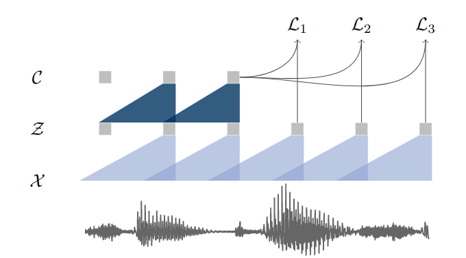
Illustration of pre-training from audio data X which is encoded with two convolutional neural networks that are stacked on top of each other. The model is optimized to solve a next time step prediction task.
Encoder
- 5 layers of 1-D causal convolutions
- Kernel sizes (10, 8, 4, 4, 4)
- Strides (5, 4, 2, 2, 2)
- 512 channels
- Activation: ReLU
- Group normalization
- Receptive field: 465
- Stride: 160
- On 16 kHz data
- Receptive field: 29.0625 ms
- Stride: 10ms
Context Network
- 9 layer of 1-D causal convolutions
- Kernel size 3
- Stride 1
- 512 channels
- Activation: ReLU
- Group normalization
- On 16 kHz data
- Total receptive field: ~210 ms
- Stride: 10ms
- Note that the context network is fully convolutional, which can be easily parallelized on modern hardware. This is different from CPC, which uses an auto-regressive model as context network.
Decoder for Pre-training
- No decoder, loss is computed on $k$ log-bilinear product between $z_{i+k}$ and $c_i$
- Requires $K$ bilinear heads: $h_1, …, h_K$
- Negative sampling (avoid collapse of representation)
- Number of negatives samples $\lambda$: 10
- Sampling distribution: $p_n$: uniform random over the same sequence
Contrastive loss for head $k$ and time step $i$:
\[\mathcal{L} = \log \sigma(z_{i+k}^\top h_k c_i) + \lambda \mathbb{E}_{\tilde{z} \sim p_n} [ \log \sigma(-\tilde{z}^\top h_k c_i) ]\]Decoder for ASR
- Classification head on lexicon + language model
- Paper: wav2letter++: The Fastest Open-source Speech Recognition System
wav2vec 2.0
wav2vec 2.0 adopts a Transformer based architecture:
- Performance: wav2vec 2.0 outperforms the SOTA model trained on 100x more labeled data
- Discretization: use Vector Quantization to map continuous representations into discrete ones
Architecture
- Input: raw waveform $x$
- Encoder: map $x$ to $z$
- Context network: map a sequence of embeddings $(z_1, …z_T)$ to a sequence of contextualized embeddings $(c_1, …, c_T)$
- Quantization Module: map continuous $z$ to discrete $q$
- Decoder
- Pre-training: no decoder / Contrastive loss + Diversity loss
- Fine tuning: ASR task (Connectionist Temporal Classification (CTC) loss)
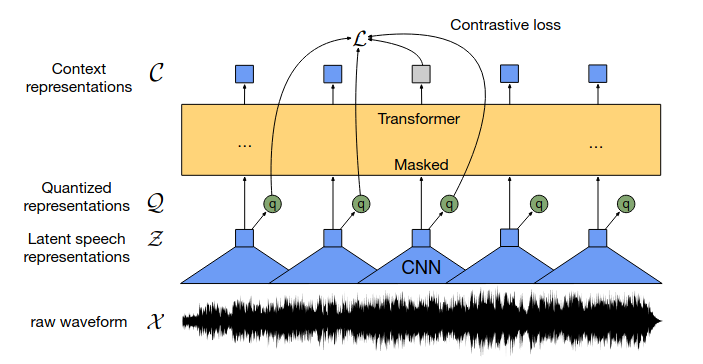
wav2vec2.0 architecture: jointly learns contextualized speech representations and an inventory of discretized speech units.
Encoder
- Temporal convolution
- Activation: GELU
- Layer normalization
Context Network
- Transformer Encoder
- Relative Positional Encoding by convolutional layer link
- Activation: GELU
- Layer normalization
- Masking: Masked Language Models (Not Causal Attention Mask)
Quantization Module
- Reading: An Illustrated Tour of Wav2vec 2.0
- Map continuous $z \in \mathbb{R}^d$ to discrete $q \in [1, …, V]^G$
- $G$: number of codebooks
- $V$: length of each codebook
- Codebook entry = discretized speech units
- Product Quantization
- Gumbel Softmax
- For computing gradient through the $\text{argmax}$ operator
- Paper: Categorical reparameterization with gumbel-softmax
- Reading: What is Gumbel-Softmax?
Decoder for Pre-training
- No decoder, $c_t$ is directly compared to $q_t$ and $\tilde{q}$ in loss function
- Contrastive loss
- similarity function: cosine similarity
- Diversity loss
- Encourage the equal use of the $V$ entries in each of the $G$ codebooks
Contrastive loss for token $t$:
\[\mathcal{L} = -\log \frac{\exp(sim(c_t, q_t)/\kappa)}{ \sum_{\tilde{q} \sim Q_t} \exp(sim(c_t, \tilde{q})/\kappa) }\]Decoder for ASR
- Linear layer which maps $c$ to vocabulary
- Loss: CTC loss
HuBERT
HuBERT is the abbreviation for Hidden unit BERT. The “Hidden unit” refers to the unobserved states in the hidden markov model, which generate the observed data. In the context of speech data, the unobserved states is the phoneme and the observed data is the raw waveform.
HuBERT is largely based on wav2vec 2.0’s architecture, but changes how discrete tokens are generated: wav2vec uses a Quantization Module, while HuBERT uses clustering. The authors mentioned that their work was inspired by the Deep Clustering paper, which proposed a framework for unsupervised learning on image data.
Architecture
- Encoder: map raw waveform to embedding $x$
- Context network: map a sequence of $X$ to a sequence of contextualized embeddings $\hat{Z}$
- First apply language model mask: $X \rightarrow \tilde{X}$
- Then apply transformer to the masked sequence: $\tilde{X} \rightarrow \hat{Z} = (\hat{z}_1, …, \hat{z}_T)$
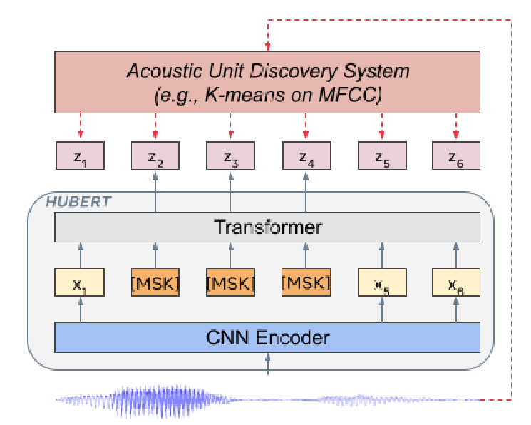
- Clustering Module $h$: map continuous representation to discrete $z$
- $Z = h(X) = (z_1, … , z_T)$
- $z_t \in [C]$, a C-class categorical variable
- Decoder
- Pre-training: no decoder / language model loss
Encoder
- Temporal convolution
- Each encoder encode 20 ms data at 16kHz sampling rate (FIV = 320)
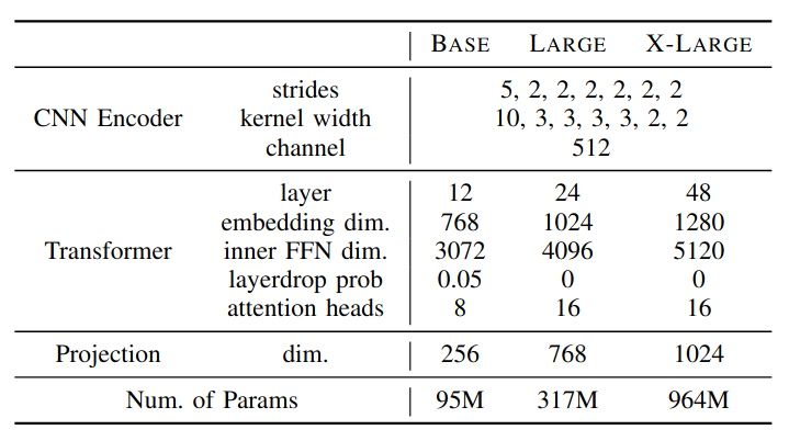
- Detailed configuration is attached below
Context Network
- Transformer Encoder
- Masking: Masked Language Models
- Detailed configuration is attached below
Clustering Module
- Clustering (k-means) could be run on MFCC features or learned representation
- A training schema could be: first initialize the cluster assignment from MFCC features, then run clustering on learned representation
- MFCC features: 100 clusters on 39-dimensional MFCC features
- Learned representation: 500 clusters on intermediate transformer layer (e.g., 9th layer from BASE HuBERT)
- Iterative Refinement: clustering model $h$ could be updated during the training
- Sampling: randomly sample 10% of the data for fitting the k-means model
Decoder for Pre-training
- No decoder, $c_t$ is directly compared to $q_t$ and $\tilde{q}$ in loss function
- Language model loss
Let $f$ be the mapping induced by the transformer. $M$ be the masking, a set of indices from a length $T$ sequence $[1, …, T]$. $X, Z$ as defined above. The loss function $L$ for masked sequence is defined as:
\[L = \alpha L_m + (1 − \alpha)L_u\] \[L(f; X,M,Z) = \sum_{t \in M} \log p_f(z_t |\tilde{X},t)\]where $L_m$ be the loss for the masked steps and $L_u$ be the loss for the unmasked steps; $p_f$ is defined as:
\[p_f(c | \tilde{X}, t) = \frac{ \exp(\text{sim}(A \cdot o_t, e_c)/\tau ) }{ \sum_{c' \in C} \exp(\text{sim}(A \cdot o_t, e_{c'})/\tau ) }\]where $A$ is the projection matrix for iteration $k$ (for reduced computation); $e_c$ is the embedding for token $c$; $\text{sim}$ is the cosine similarity; $\tau$ is the temperature, which is set to 0.1.
Ablation Study
- HuBERT achieves better WER when clustering with learned representation (TABLE IV, TABLE V)
- Deeper transformer layer generally achieved better representation (Figure 2)
- HuBERT achieves better WER when pre-training with $\alpha = 1$, i.e., only predict masked tokens (TABLE V)