Contrastive Learning
This post is mainly based on
- Lilian Weng’s blog on Contrastive Learning
- Representation Learning with Contrastive Predictive Coding, 2018
- A Simple Framework for Contrastive Learning of Visual Representations, ICML 2020
Contrastive learning can trace its roots back to the siamese network. Siamese networks are generally motivated by the need to identify if the a pair of input is originating from the same source. For example, signature verification or face verification. It was sometimes referred to as “metric learning” or “similarity learning”.
Siamese Network
Signature Verification
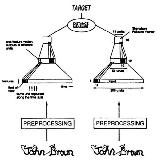
In the 1993 paper, the siamese network is used for signature verification. It maps a pair of inputs to a pair of embeddings. The output layer measures the cosine similarity between two embeddings. For signature pair from the same individual, the cosine angle is assigned as $1.0$. For signature pair from different individuals, the cosine angle is assigned as $-0.9$ or $-1.0$. Therefore, the optimization is pulling similar images into same direction in latent space while pushing different images opposite directions.
Face Verification
The 2005 paper uses siamese network for face verification. To my knowledge, the term “Contrastive Loss” is first pinned down in this paper. Given a training data $(Y, X_1, X_2)$, where $Y = 0$ if the the images tuple belongs to the same person (genuine) and $Y=1$ otherwise (impostor). Let $E_W$ be the energy function given the network parameter $W$,
\[E_W(X_1, X_2) = \| G_W(X_1) - G_W(X_1) \|_2\]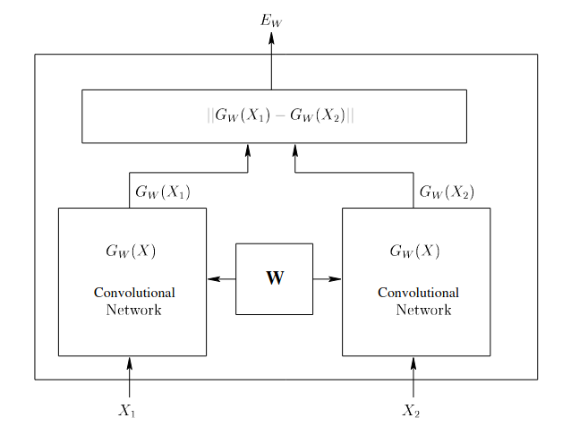
The contrastive loss function is defined as:
\[\mathcal{L}() = (1-Y) L_G(E_W(X_1, X_2)) + Y L_I(E_W(X_1, X_2))\]where $G$ stands for genuine pairs and $I$ stands for impostor. We can choose $L_G$ to be monotonically increasing, and $L_I$ to be monotonically decreasing. Under this loss function, the optimization will decrease the energy $E_W(X_1, X_2)$ of genuine pairs and increase the energy $E_W(X_1, X_2)$ of impostor pair. Hence $E_W$ behave like a similarity measure.
Note that in these early works, the goal is learning a good similarity measure rather than learning a good representation.
Contrastive Predictive Coding
Prior to Contrastive Predictive Coding (CPC), there are some works on contrastive loss, for example: Triplet Loss, Lifted Structured Loss and N-pair Loss. However, they either suffered from efficiency problems or the experiments are not performed on large datasets like ImageNet.
CPC is different from the above works due to:
- It’s a general model and compatible with images, speech, natural language and reinforcement learning data
- Its loss function is more theoretically sound: maximizing mutual information
- It beat previous SOTA unsupervised methods by a large margin on LibriSpeech and ImageNet
They authors mentioned that they are motivated by negative sampling/contrastive loss technique of Word2Vec and the triplet loss mentioned above.
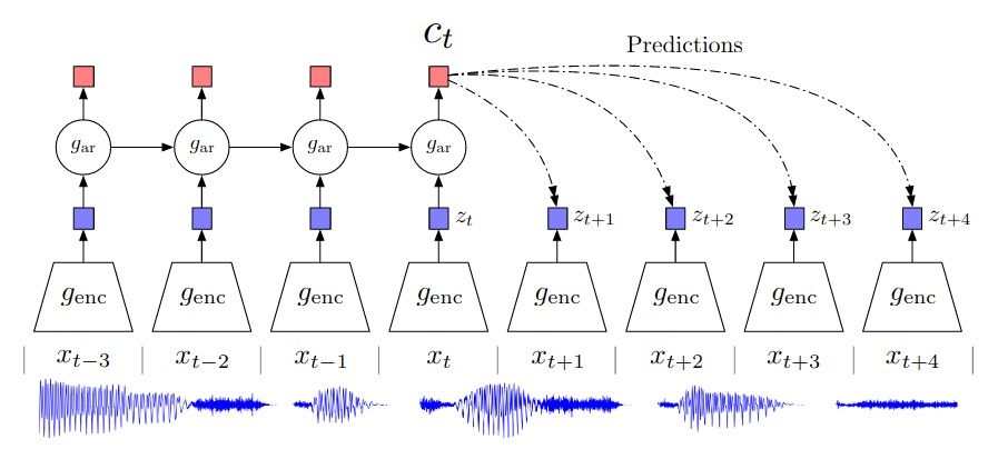
Data is first first split into chunks: $…, x_{t-2}, x_{t-1}, x_t, x_{t+1}, x_{t+2}, …$ and up to $x_t$ is available to model. The encoder $g_{enc}$ maps $x_i$ to $z_i$. The authors uses a strided ResNet CNN as encoder. The autoregressive model $g_{ar}$ take its previous state and $z_i$ to compute its current state and output the context vector $c_t$. The autoregressive model $g_{ar}$ could be an LSTM or GRU. The loss function is InfoNCE loss and it can be shown that minimizing InfoNCE is equivalent to maximizing a lower bound on mutual information $I(x;c)$ between future data $x_i$ and current context $c_t$.
\[I(x;c) = \sum_{x,c} p(x,c) \log \frac{p(x|c)}{p(x)}\]Mutual information (MI) measures the mutual dependence between the two variables. Maximizing MI requires the underlying encoder $g_{enc}$ and autoregressive model $g_{ar}$ extract features that consist of shared information from the “past” and the “future”. Why we care about this shared information? It comes from the assumption that each chunk of data $x_i$ is generated from some latent variables $z$. Some $z$ generate low-level and local information; other $z$ generate high-level and global information. The optimization force the model to extract features that are related to the high-level and global $z$. Such feature contains information that spans multiple time steps and is useful for predicting task. The paper discussed this motivation in section 2.1 in details.
Contrastive Predictive Coding
Given previous architecture of $g_{enc}$, $g_{ar}$, define a log-bilinear model $f_k$:
\[f_k(x_{t+k}, c_t) = \exp(z^\top_{t+k} W_k c_t)\]The CPC model will learn a different $W_k$ for each look ahead step $k$.
Our claim is that $f_k$ measures the dependency between the future $x_{t+k}$ and the past $c_t$ (will show why later):
\[f_k(x_{t+k}, c_t) \propto \frac{p(x_{t+k}|c_t)}{p(x_{t+k})}\]Under this setting, both $z_t$ and $c_t$ learns a representation of data $x$. The different is: $z_t$ only contains information for current data $x_t$, while $c_t$ contain information up to time step $t$ learned by the autoregressive model.
InfoNCE Loss
Recall that under contrastive learning framework, we have one positive example and no less than one negative example. Let $x_+$ be the positive example at $k$ look ahead step: $x_+ = x_{t+k}$. Sample negative examples $x_-$ to construct a batch: $X = \{ x_1, …, x_N \}$. $X$ contains one positive sample $x_+$ and $N-1$ negative sample $x_-$. The InfoNCE Loss is defined as,
\[\ell_N = -\mathbb{E}_X \left[ \log \frac{f_k(x_+, c_t)}{ \sum_{x_j \in X} f_k(x_j, c_t) } \right]\]If we assume each $x_j \in X$ represent one class and $x_+$ is the correct class. The $\ell_N$ becomes the cross entropy loss for $x_+$. The probability of predicting the correct class $x_+$ given context $c_t$ is:
\[\begin{align} p(x_+ | X, c_t) &= \frac{p(x_+, X, c_t)}{p(X, c_t)} \\ &= \frac{p(x_+, X, c_t)}{\sum_j p(x_j, X, c_t)} \\ &= \frac{p(x_+ | c_t)p(X)}{\sum_j p(x_j | c_t)p(X)} \\ &= \frac{p(x_+ | c_t)\prod_{x \not= x_+} p(x)}{\sum_j p(x_j | c_t) \prod_{x \not= x_j}p(x)} \\ &= \frac{\frac{p(x_+ | c_t)}{p(x_+)}}{\sum_j \frac{p(x_j | c_t)}{p(x_j)} } \\ \end{align}\]Note that the paper does not provide a derivation and the above is my understanding: the third and forth steps assumes independence of each $x_j$ and the last step is obtained by dividing both numerator and denominator by $p(X)$. Recall that $\ell_N$ is defined as $\ell_N = \frac{f(x_+, c_k)}{\sum f(x, c_k)}$. Therefore, for optimal $f_k$,
\[f_k \propto \frac{p(x_+ | c_t)}{p(x_+)} = \frac{p(x_{t+k} | c_t)}{p(x_{t+k})}\]For optimal $f_k$, the author show in appendix A.1 that, $\ell_N = p(x_+ | X, c_t) \geq -I(x_+, c_t) + \log(N)$. Hence,
\[I(x_{t+k}, c_t) \geq -\ell_N + \log(N)\]where $\log(N)-\ell_N$ can be viewed as a lower bound of mutual information. Note that this idea is similar to the variational inference: to minimize the KL-divergence between $p,q$, we maximize the Evidence Lower Bound (ELBO).
Personally, I am a little bit uncomfortable about the cross entropy argument since it appears to imply that there are $N-1$ negative classes and each time you can sample exactly one $x_-$ into each negative class.
Experiments
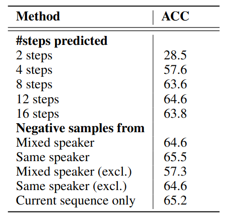
The audio experiments are based on 100-hour subset of the publicly available LibriSpeech dataset. The result shows that features learned by CPC significantly outperformed handcrafted features (MFCC) and random features. It almost achieve comparable level of performance as supervised model on speaker classification task. The ablation studies shows that look ahead step $k$ affects the learned representation: short steps learns trivial features that are not really useful in downstream tasks, while long steps may result in performance deterioration. One can imagine the choice of $k$ depends on the downstream tasks.

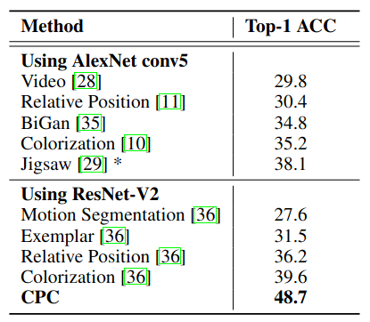
Due to there is no intrinsic order in image data, some engineering works are required for CPC to work on 2D images. The CV experiments show that CPC beat previous Pretext tasks based SSL methods by a large margin. However, CPC still lags behind supervised learning by a large margin (ResNet-152 can achieve 81.3% Top-1 ACC, source). This gap is gradually narrowed by future SSL methods.
Discussion
The optimization goal of this paper is maximizing mutual information. Another work based on this principle is Learning Representations by Maximizing Mutual Information Across Views. However, whether maximizing mutual information should be the optimization goal is questioned in the paper On Mutual Information Maximization for Representation Learning. Future SSL methods which does not follow this principle (e.g., SimCLR and MoCo) also achieve SOTA performance.
SimCLR
SimCLR belongs to another class of contrastive learning methods that relies on heavy data augmentation. Recall that CPC divide $X$ into many little chunks $ …, x_{t-2}, x_{t-1}, x_t, x_{t+1}, x_{t+2}, … $. For image data that does not have an intrinsic order, CPC will assign one (top-down and bottom-up). This approach has a benefit: positive examples are generated from one training sample $X$ and we don’t need a deep understanding of how to augment data. This advantage is crucial in field that involves high dimensional time series data.
In comparison, SimCLR generate positive examples by augmenting one training sample $X$ into two versions. My understanding is it is primarily used CV field where we have a good understanding of what data transformation is invariant. For fields like NLP, how to augment data without changing its meaning is less obvious (e.g., deletion of the word “NOT” can completely reverse the meaning of a sentence). There are some works that propose translating a sentence into another language and then translate back, but this perhaps makes data augmentation very expensive (need a powerful language model and translation hard to parallelize).
Discussions on how to make this type of methods work can be found in Lilian Weng’s blog:
SimCLR Framework
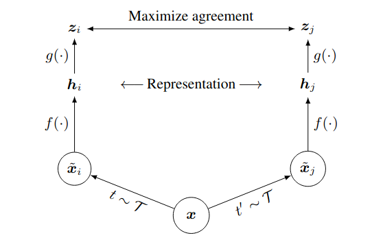
SimCLR framework comprises four major components:
- Stochastic data augmentation module
- Random cropping, random color distortions, and random Gaussian blur
- augment $x$ into two verions: $\tilde{x}_i$ and $\tilde{x}_j$
- Base encoder $f(\cdot)$
- ResNet
- $h_i = f(\tilde{x}_i)$
- Projection head $g(\cdot)$
- MLP with one hidden layer
- $z_i = g(h_i)$
- Contrastive loss function $\ell_{i,j}$
- Do not sample negative examples explicitly
- Given a batch of $N$ images, augmentation produced $2N$ images
- The rest of $2(N − 1)$ are negative examples
- Define $\operatorname{sim}(u, v)$ as cosine similarity
Loss function:
\[\ell_{i,j} = -\log \frac{\exp(\operatorname{sim}(i,j) / \tau)}{ \sum_k \mathbb{1}_{k \not= i} \exp(\operatorname{sim}(i,k) / \tau) }\]where $\tau$ is a temperature parameter. This loss is computed across all positive pairs in a mini-batch.
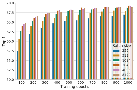
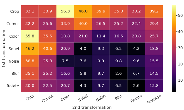
SimCLR replaced the memory back by large batch size (up to 8192) and longer training (1000 epochs). This requires a lot of computation resource, quote With 128 TPU v3 cores, it takes ∼1.5 hours to train our ResNet-50 with a batch size of 4096 for 100 epochs. Data augmentation is essential: the composition of random cropping and random color distortion achieve around 56% accuracy, while other combinations of data augmentation are lagging behind.
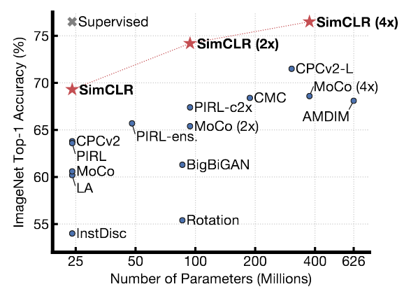
SimCLR achieve SOTA in 2020, beating CPCv2 by a large margin on ImageNet Top-1 ACC without tuning.
I was a bit concern about the inductive bias of the architecture as cropping seems to implies that SimCLR relies on object centric datasets like ImageNet and CIFAR. However, performance of SimCLR is good on PASCAL VOC (random crop may result in crop out of 2 different classes of object on those object detection datasets). It is possible that Global and local views cropping helps to reduce this bias.