DL Generalization
- On Large-Batch Training for Deep Learning: Generalization Gap and Sharp Minima, ICLR 2017
- Understanding deep learning requires rethinking generalization, ICLR 2017
Generalization in deep learning is still not well understood and the two paper listed above explore two directions.
The first paper studies the relationship batch size and generalization. This paper provides experimental evidence on batch size, sharpness of minimizer and generalization gap. They found that the lack of generalization ability is due to the fact that large-batch methods tend to converge to sharp minimizers of the training function. Additional discussions on large batch methods can be found at the Learning Rate vs Batch Size post.
The second paper finds that traditional statistical learning theory fail to explain why large neural networks generalize well. Their experiments suggest that the model capacity of neural network is high enough to memorize random noise. They also find that network architecture has a much higher impact on generalization ability than explicit regularization.
Why Large-Batch Leads to Poor Generalization
Assumptions
- Large batch (LB) methods lack the explorative properties of small batch (SB) methods. Therefore, they tend convergence to local minima closer to the initial point
- SB and LB methods converge to qualitatively different minimizers with differing generalization properties
Sharpness of Minimizer and Generalization Error
The concept of a “flat minimum” in neural network was discussed in a 1997 paper Flat Minima. The authors mentioned that Bayesian argument suggests that flat minima correspond to “simple” networks and low expected overfitting. They define flat minimum as a large region of connected acceptable minima, which leads to almost identical neural network output.
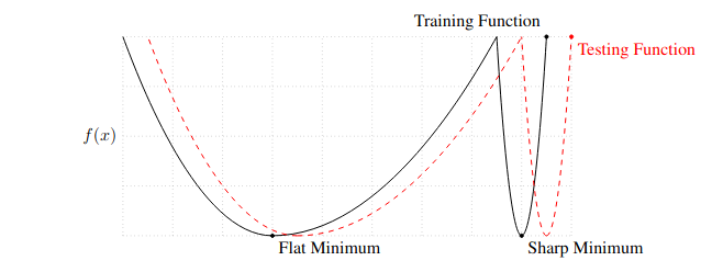
Conceptual Sketch of Flat and Sharp Minima. The Y-axis indicates value of the loss function and the X-axis the variables (parameters)
The above figure shows the intuition of why flat minimum should be preferred in optimization:
- Due to data set $\{x\}$ is sampled from the population, our estimation of loss function only approximate ground truth loss function
- Flat Minimum: training loss minima likely correspond to low testing loss
- Sharp Minimum: training loss minima likely correspond to higher testing loss, due to rapid changes in its neighborhood
Batch Size, Sharpness and Generalization Error
The experiment is as follow: for different batch sizes, optimize the network from randomly initialized weight and then measure the sharpness of minima. The sharpness of minima is measures by a numerical approximation of the magnitude of the eigenvalues of $\nabla^2 f(x)$ (For dense matrix, the exact solution is too expensive to compute link). For more details, please refer to Metric 2.1 of the first paper.
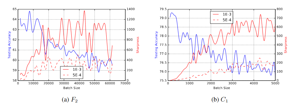 Testing Accuracy and Sharpness v/s Batch Size. x-axis: batch size used for training the network for 100 epochs; left y-axis: testing accuracy; right y-axis: sharpness; result are reported for two learning rates: 1e-3 and 5e-4. F2: Fully Connected network on TIMIT dataset; C1: Shallow Conv Net on CIFAR-10 dataset; details in Appendix B.
The above result support the view that poor generalization is caused by large-batch methods tend to converge to sharp minimizers.
Rethinking Generalization
Neural networks are can be trained in over-parameterized setting: number of parameters > number of training data. In traditional machine learning, an over-parameterized model is almost certainly doomed to fail due to overfitting. However, many over-parameterized neural network work surprisingly well in practice and can achieve very small difference between training and testing error.
The authors of the second paper conduct empirical studies and show that statistical learning theory fails to explain why over-parameterized network generalized well. For this post, we will present the paper result first and then explain why statistical learning theory fails to explain the generalization gap.
Effective Capacity of Neural Network
To estimate the model capacity, the authors run a series of randomization tests on CIFAR10 dataset. I consider this as analogous to VC-dimension: if model has high capacity (e.g., VC-dimension $\geq n$), then it should be able to shatter a dataset of size $n$, or equivalently to fit a dataset $\{ (x_i, y_i) \}_{i=1}^n$ for any label $y_i$ with zero training error. The experiments can be classified into 2 categories: label randomization and data randomization.
Label Randomization
- True labels: the original dataset without modification
- Partially corrupted labels: independently corrupt labels with probability $p$
- Random labels: all the labels are replaced with random ones
Data Randomization
- Shuffled pixels: a random permutation of the pixels is chosen and then the same permutation is applied to all the images in both training and test set
- Random pixels: a different random permutation is applied to each image independently (distribution of each image is preserved)
- Gaussian: A Gaussian distribution (with matching mean and variance to the original image dataset) is used to generate random pixels for each image (distribution of each image is removed)
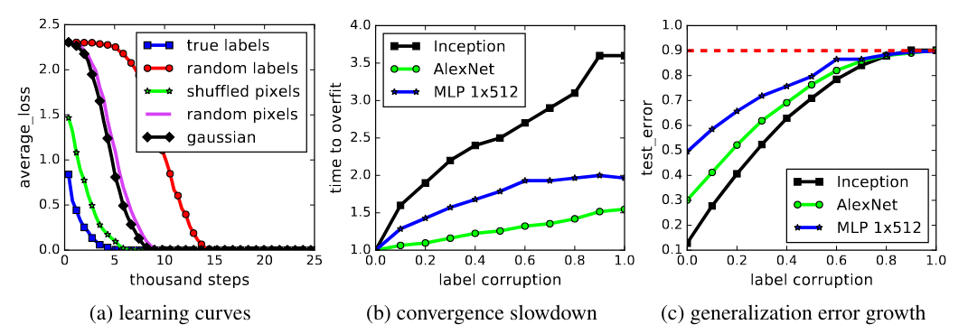
Fitting random labels and random pixels on CIFAR10. (a) shows the training loss of various experiment settings decaying with the training steps. (b) shows the relative convergence time with different label corruption ratio. (c) shows the test error (also the generalization error since training error is 0) under different label corruptions.
Figure (a)’s label randomization test shows that
- Deep neural networks easily fit random labels
- The effective capacity of neural networks is sufficient for memorizing the entire data set
Figure (a)’s data randomization test shows that
- Despite their engineered architecture for processing local spartial structure, CNNs (Inception, AlexNet) can memorize random noise input
Figure (b) shows that
- Optimization on random labels remains easy, since training time increases only by a small constant factor
Figure (c) shows that
- By vary the amount of randomization, the authors create a range of intermediate learning problems
- The steady deterioration of the generalization error shows that neural networks are able to capture the remaining signal in the data, while memorize the noisy part using brute-force
Statistical Learning Theory
VC Dimension and Rademacher Complexity
We previously discussed Empirical Risk Minimization (ERM) in this post. The key finding is that: for a finite size function class $\mathcal{F}$, with probability $1-\delta$, the generalization gap is determined by $| \mathcal{F} |$:
\[| \hat{R}_n(f) - R(f) | \leq \sqrt{\frac{B^2 \log(2| \mathcal{F} |/\delta)}{2n}} = g(| \mathcal{F} |)\]where $g$ is a function of $| \mathcal{F} |$.
There is another version of the ERM theorem for infinite size function class $\mathcal{F}$, which uses the VC-dimension. It could be written as:
\[| \hat{R}_n(f) - R(f) | \leq g( \operatorname{VC-dim}(\mathcal{F}))\]Also for Rademacher Complexity
\[| \hat{R}_n(f) - R(f) | \leq g( \operatorname{Rad}(\mathcal{F}, S, \ell))\]where $\operatorname{Rad}(\mathcal{F, S})$ is jointly determined by the function class $\mathcal{F}$, the sample $S=(z_1, z_2, \dots, z_m) \in Z^m$ and the loss function $\ell$.
The author does not elaborate on the shortcomings of the above measure in details. My understanding is
- Bounds by VC dimension
- Bounds by VC dimension only consider $\mathcal{F}$, where figure (c) shows that generalization likely also related to dataset $S$
- The authors can force the generalization error of a model to jump up considerably without changing the model, its size, hyperparameters, or the optimizer
- Bounds by Rademacher Complexity
- If network can fit random labels on a dataset $S$, then $\operatorname{Rad}(\mathcal{F}, S, \ell) = 1$.
- $\operatorname{Rad}(\mathcal{F}, S, \ell) = 1$ implies overfitting / poor generalization
- Bounds by Rademacher Complexity is likely too loose to provide any useful information on generalization error of neural network
- Too adversarial
- The above error bounds are derived using concentration inequality, which means that they need to handle arbitrary distribution
- This setting is probably too adversarial
Some ideas are borrowed from this stackexchange question.
Uniform Stability
Error bound provided by uniform stability can be found in Definition 5 and Theorem 11 of Stability and Generalization paper:
\[| \hat{R}_n(f) - R(f) | \leq g( \beta(\mathcal{F}) )\]where $\beta$ measure of stability (e.g., uniform stability) of a learning algorithm $A$. $\beta$ can be think as the highest performance deterioration caused by deleting or modifying any single data point.
The authors argue this error bound is also problematic since it is solely a property of the algorithm, which does not take into account specifics of the data or the distribution of the labels.
The Role of Regularization
- Explicit regularization
- Data augmentation
- Weight decay (equivalent to L-2 regularizer on the weights)
- Dropout
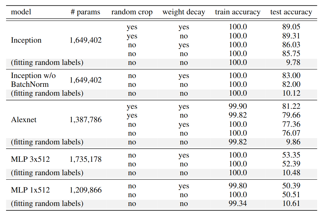
The training and test accuracy (in percentage) of various models on the CIFAR10 dataset. Performance with and without data augmentation and weight decay are compared. The results of fitting random labels are also included.
In traditional machine learning, regularization (e.g., L2 regularization) help confine learning to a subset of the hypothesis space with manageable complexity. By adding an explicit regularizer, say by penalizing the norm of the optimal solution, the effective Rademacher complexity of the possible solutions is dramatically reduced.
However, explicit regularization seems to play a different role in neural network. The above result shows that network architecture plays a much important role in generalization gap than explicit regularization. Switching from Inception to MLP result in a generalization gap jump from 15% to nearly 50%. However, turning off random crop or weight decay only result in single digits increase in generalization gap.
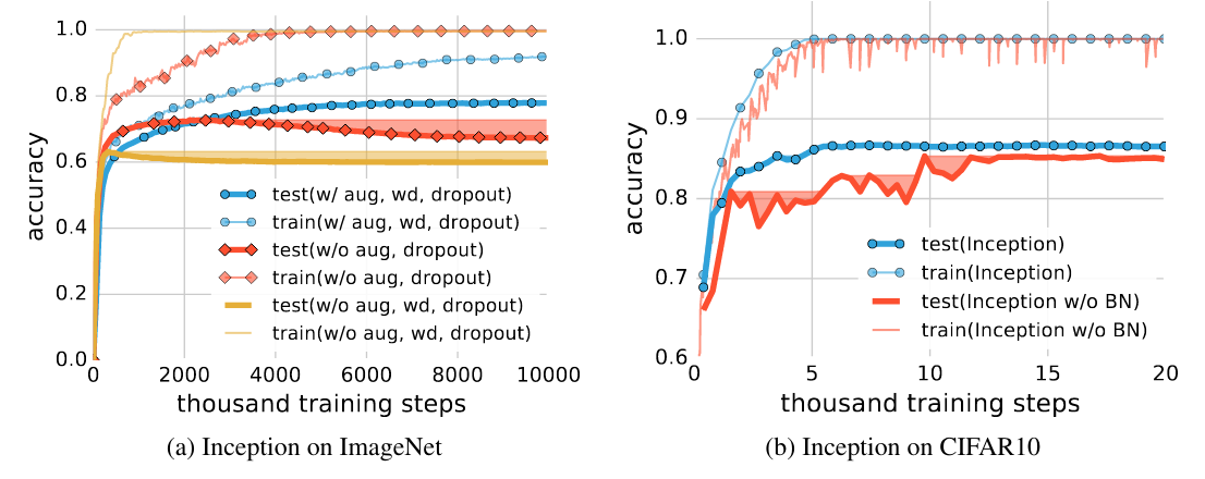
Effects of implicit regularizers on generalization performance. aug is data augmentation, wd is weight decay, BN is batch normalization. The shaded areas are the cumulative best test accuracy, as an indicator of potential performance gain of early stopping. (a) early stopping could potentially improve generalization when other regularizers are absent. (b) early stopping is not necessarily helpful on CIFAR10, but batch normalization stablize the training process and improves generalization.
On larger dataset, explicit regularization seems to become more important (Imagenet had larger images (224 pixels, 160GB) and more categories (1000) compared to CIFAR10). Turning off regularization result in regularization gap increase from around 10% to 40%. Batch normalization stablize the training, but has limited impact on the generalization gap.