Attention Mechanism
This post is mainly based on
- Neural Machine Translation by Jointly Learning to Align and Translate, ICLR 2015
- Attention Is All You Need, NIPS 2017
- Attention and Memory in Deep Learning and NLP
- Peter Bloem’s blog
- The Illustrated Transformer
Attention Mechanism is a quite overloaded term: it has been used in different ML model. This goal of this post is resolve those confusions. This post will be structured as a chronological review:
- Before 2014, RNN without Attention
- 2014 - 2017, RNN with Attention
- After 2017, Self-Attention / Transformer
This post does not discuss Transformer. For discussions on Transformer, check this post.
RNN
Consider Neural Machine Translation (NMT) task: NMT is a sequence to sequence (seq-2-seq) modeling problem: for example, given a sequence of English words as input, the model should output is a sequence of French words. Before transformer, RNN is the benchmark model for NMT tasks. In practice, researchers found RNNs have the “forgetting” problem: given a long sentence, RNNs tends to forget the information at the beginning of the sentence.
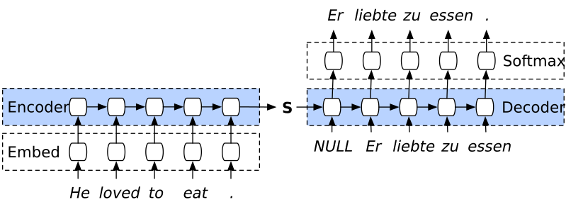
RNN uses a encoder-decoder architecture to model the seq-2-seq problem as shown above. The encoder encode the English sentence into hidden states and decoder use the last hidden state of encoder to generate French words. Researchers hypothesize the “forgetting” problem is due to the decoder generate the entire translation solely based on the last hidden state from the encoder. The last hidden state needs to encode the information of the entire sentence, which is theoretically possible but hard to achieve in practice. If you look at a human translator, they don’t just take a glimpse at the English sentence, memorizing everything, tossing the English sentence away and start to write French.
In 2014, researchers found that input reversing (passing the sentence in a reverse order to the encoder), and input doubling (passing the sentence to the encoder twice) improves the performance of RNN, which hinted the problem could be encoding everything into one state.
RNN with Attention
The RNN with Attention architecture was introduced by Bahdanau and Bengio in 2014. The Intuition is that model should be able to access different words from source sentence durning translation, just like human translator often refer back to specific words in the source sentence. Based on this intuition, the authors add a learnable module that determines which hidden state should be feed to the decoder. Instead of look at the last hidden state, the model can access all hidden state and decide which part is important for the next French word.
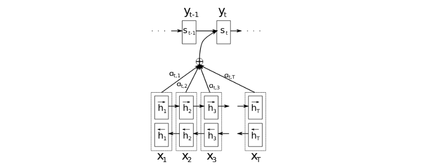
The graphical illustration of the proposed model trying to generate the t-th target word $y_t$ given a source sentence $(x_1, x_2, … , x_T )$.
Decoder step
- Alignment model
- Alignment model $a$ is a learnable network
- $e_{ij}=a(s_{i-1}, h_j)$: $a$ takes previous decoder state $s_{i-1}$ and any encoder state $h_j$ and compute their similarity $e_{ij}$
- $\alpha_{ij} = \frac{\exp(e_{ij})}{\sum_k \exp(e_{ik})}$: the alignment score $\alpha_{ij}$ is compute as the softmax of $e_{ij}$
- $c_i = \sum_{j=1}^{T} \alpha_{ij} h_j$: the context vector $c_i$ is computed as a weighted sum of encoder state $h_j$
- RNN
- Append context vector $c_i$ and vector of previous translated word $y_{i-1}$
- $s_i = f(s_{i−1}, y_{i−1}, c_i)$: compute decoder state $s_i$
- Sample next word $y_i \sim g(s_{i})$
$\alpha_{ij}$ can be viewed as attention score and act as an information selection filter: given the previous translated word, which word in the source sentence is important. Below is an example of the model assigning attention score to European Economic Area in reverse order.
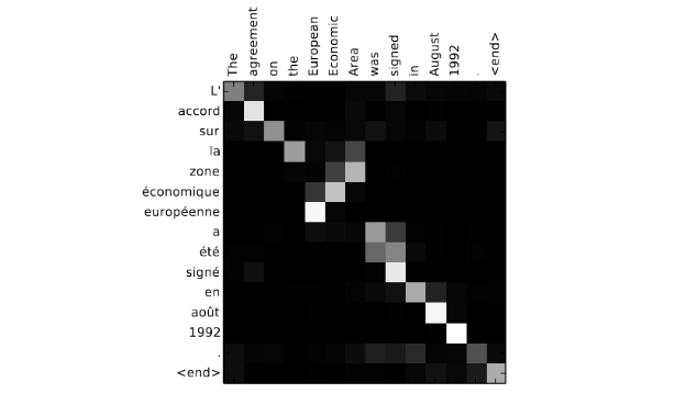
Alignment score visualization (0: black, 1: white). The x-axis and y-axis of each plot correspond to the words in the source sentence (English) and the generated translation (French)
The context vector $c_i$ is s a distributed representation of all encoder hidden states. The term “context” means “taking the meanings of words in source sentence that are relevant to the target translation word into consideration”. This architecture yields the following model:
\[p(y_i|y_1, . . . , y_{i−1}, x) = g(y_{i−1}, s_i, c_i)\]Compared the above equation to RNN without attention $p(y_i|y_1, . . . , y_{i−1}, x) = g(y_{i−1}, s_i, h_T)$. Note that, With attention mechanism, information from the source sentence is not required to be all encoded into one state $h_T$. Rather, the model can selectively access information from the source sentence by $c_i$.
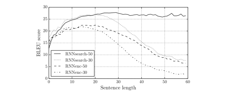
This architecture significantly increase the quality of long sentence translation. As shown below, RNN with Attention hold it performance whereas RNN without Attention saw a significant drop in performance after sentence length exceed 40.
Self-Attention
Prior to 2017, attention is mainly used as auxiliary module in the RNN architecture. The model that performs the heavy lifting work (encoder, decoder) is still the RNN. However, RNN is not easily parallelizable, and this type of architecture cannot scale up efficiently (e.g., >10GB of uncompressed text). To removed the RNN, Vaswani et al. from Google designed a new architecture called Transformer, which operate solely on attention.
Note that there are different types of attentions in Transformer:
- Self-Attention
- Causal-Attention
- Cross-Attention
We will describe the Self-Attention here.
A Self-Attention is a seq-2-seq operation. What makes Self-Attention useful is: when computing the embedding of the target vector, Self-Attention can take the information from other vectors in the sequence into consideration.
Consider a traditional word embedding, e.g., Word2Vec. Word2Vec maps a token to a vector based on the token itself: it cannot extract information from other tokens in the sentence. A Self-Attention operation is different: it takes a sequence of input word vectors $(x_1, x_2, …, x_t)$ and maps it into a sequence of contextualized word embedding $(z_1, z_2, …, z_t)$. The contextualized word embedding compute the vector for each token in context of the sentence.
What is the propose of contextualized word embedding? Consider the source word “bank”. Bank is a homonym: it could mean a financial institution or an area bordering a lake or river. The semantics of bank is important since two of its meaning may correspond to different words in target language. To determine the semantics of bank, one needs to consider the words around it.
Toy Example
Suppose $z_i$ is computed as a weighted sum of $x_i$:
\[z_i = \sum_j w_{ij} x_j \tag{1}\]where the weight $w_{ij}$ measures the similarity between the $i$-th and $j$-th word. The simplest way to measure similarity is to use a dot product:
\[w'_{ij} = x_i^{\top} x_j \tag{2}\] \[w_{ij} = \frac{\exp(w'_{ij})}{\sum_k \exp(w'_{ik})}\]Recall the “bank” example, the dot product \(w'_{ij} = x_i^{\top} x_j\) serves this “compute the meaning in context” function. In our toy example, the weight $w_{ij}$ modifies the original word embedding, such that the transformed embedding is more aligned with the content around it.
Transformer
Transformer basically implemented a more complex version of our Toy Example framework:
Let’s first compute some values in an intermediate step:
- Query: $q_i = W_q x_i$
- Key: $k_j = W_k x_j$
- Value: $v_j = W_v x_j$
Compute the weight and normalized weight from the intermediate step:
\[w'_{ij} = q_i^{\top} k_j\] \[w_{ij} = \operatorname{softmax}(w'_{ij})\]Compute output embedding $z$:
\[z_i = \sum_j w_{ij} v_j\]The connection between Transformer and our Toy Example is:
- Query is a linear transformation applied to $x_i$ of $\text{Equation } (2)$
- Key is a linear transformation applied to $x_j$ of $\text{Equation } (2)$
- Value is a linear transformation applied to $x_j$ of $\text{Equation } (1)$
These linear transformations project word vectors $x_i$ onto higher dimensions, so that latent space of the input vector (e.g., produced by embedding layer or previous self-attention layer) can be disentangled and used for more proposes (e.g., semantic, syntactic). Training a Transformer search the space of $W_q, W_k, W_v$ such that the projections become meaningful in some NLP tasks.
Summary
To highlight connections between CNN, RNN, and Transformer.
CNN vs RNN: An RNN can be viewed as CNN with variable depth, but same kernel across all layers
RNN w Attention vs Transformer: The Attention module in RNN only assign weights to the input sequence. Attention in Transformer both compute weights ($W_q, W_k$) and meanings ($W_v$).
CNN vs Transformer: Transformer can be viewed as a generalized CNN. CNN’s kernels are trained and their weights cannot be changed at inference. Transformer’s kernel weights can change at inference: the weights depend on the input.