Causal Inference
This post is mainly based on
This post is a high level summary of [Causal Inference I] taught by Prof. Elias Bareinboim. If you have no background on Causal Inference, Brady Neal’s course is a good place to start.
Causal Inference
Causal Inference is a relative new area of research compared to well established field like statistics. The goal is to formally and mathematically study the cause and effect from observational data (or interventional data). The difference between Causal Inference and Statistics is:
- Causal Inference: study causal relationship
- Statistics: study associational relationship
For a very long time, the scientific field neglect studying “cause” or “effect.” We were taught “Correlation is not causation” from our Statistics 101 course with good reasons: the rooster’s crow correlate with, yet not cause the sunrise. However, this neglection causes problems: with just Statistics in our toolbox, we cannot answer the question of whether cigarette smoking causes a health hazard.
Fortunately, in clinical research, we can use randomized controlled trails (RCT) to pin a causal relationship. However, there are cases where an RCT is unethical, or simply impossible. For example, we cannot conduct an RCT on smoking since it is unethical to force a non-smoker to begin this habit. However, if we have observational data, Causal Inference may be able to answer this question (we use the term “may”, since whether we can identify the causal effect depends on the data we have and the assumptions we make). In fact, RCT can be viewed as a special case of “Adjustment by Direct Parents” or “Back-door Criterion.”
Causal Hierarchy
Observation vs Intervention
We begin from distinguishing observational and interventional distribution.
Suppose that, everyday, we make an observation at dawn, where the sun rise with probability 0.5. The rooster’s crow $R$ correlate with the sunrise $S$. The joint distribution $P(S, R)$ is an observational distribution:
| $S$ = 0 | $S$ = 1 | |
| $R$ = 0 | 0.5 | 0 |
| $R$ = 1 | 0 | 0.5 |
Suppose we kill the rooster for scientific advancements. Now rooster crow with probability 0, but the sun still rise. The joint distribution $P(S, do(R=0))$ is an interventional distribution:
| $S$ = 0 | $S$ = 1 | |
| $do(R = 0)$ | 0.5 | 0.5 |
The $do$-operator indicate interventions. However, we need Structured Causal Model (SCM) to formally define it.
Pearl’s Causal Hierarchy
| Layer | Distribution | Symbolic Query | Activity | Example |
| 1 | Associational | $P(y|x)$ | Seeing (Supervised learning) | What does the rooster tell about sun? |
| 2 | Interventional | $P(y|do(x))$ | Doing (Reinforcement learning) | If I kill the rooster, will the sun rise? |
| 3 | Counterfactual | $P(y_x| x’, y’)$ | Imagining (Counterfactual analysis) | The rooster is dead; what if I did not kill the rooster? Will the sun rise? |
Causal Inference = answer symbolic queries across layers of the Causal Hierarchy.
Structured Causal Model
To move around layers of Causal Hierarchy, we need a framework to define the ground truth world. Structured Causal Model (SCM) is such a framework.
An SCM $\mathcal{M}$ is a 4-tuple $<V, U, \mathcal{F}, P(u)>$, where
- $V = \{ V_1, …, V_n \}$, set of $n$ endogenous variables
- $U = \{ U_1, …, U_m \}$, set of $m$ exogenous variables
- $\mathcal{F} = \{ f_1, f_n\}$, set of function determining $V$
- $v_i = f_i(pa_i, u_i)$, value of endogenous variables are determined by function $f$
- $pa_i \in V$, endogenous input variables
- $u_i \in U$, exogenous input variables
- $p(u)$, distribution over $U$
Key takeaways
- Endogenous variables are measurable; exogenous variables are not measurable
- $V$ are deterministic given we know $u, pa$
- Randomness of SCM comes from the distribution of $U$
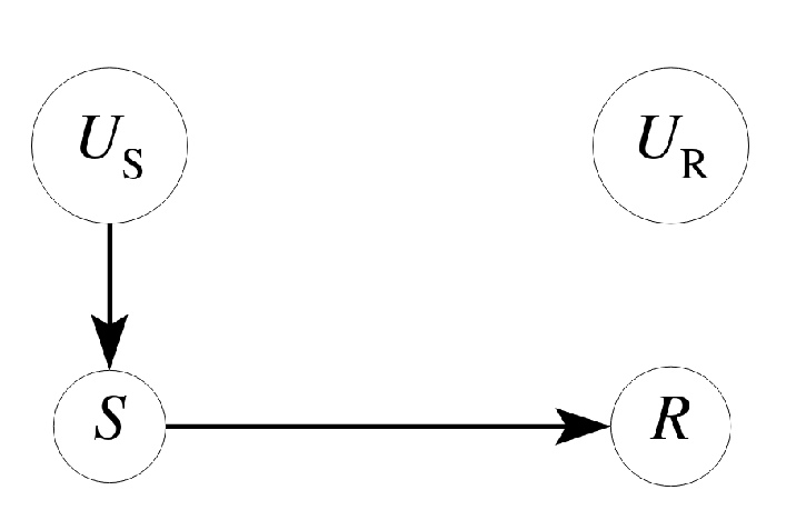
Recall the rooster vs sun example:
- $V = \{ R, S \}$
- $U = \{ U_S, U_R \}$
- $\mathcal{F} = \{ f_R, f_S\}$
- $f_R(u_r, s) = s$
- $f_S(u_s) = u_s$
- $p(u): P(u_s) \sim \text{Bernoulli}(0.5) $
Writing everything in terms of SCM is cumbersome. Observe that each SCM induces a graphical model $G$, called causal diagram.
- Each $V_i$ induced an observable node
- Each $U_i$ induced an unobservable node
- Each $f_i$ induced a set of directed edges between nodes
The rooster vs sun SCM induced the below causal diagram:
Causal diagram provides certain advantages
- Graphical model automatically implies Markov property
- d-separation can be used to evaluate the conditional independence between variables
Topics of Causal Inference
Identification Problem
The causal effect of X on Y is identifiable, if $P(y | do(x))$ can be computed from causal diagram $G$ and observational data $P(v)$.
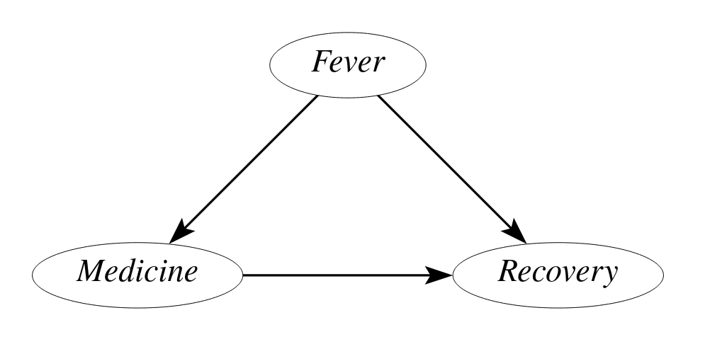
Confounding Bias
The association between outcome $Recovery$ and query variable $Medicine$ is a mixture of
- Effects from query variable $Medicine$
- Effects from confounding variable $Fever$
RCT, Adjustment by Direct Parents or Back-door Criterion can be used to isolate the effect from the query variable.
Do-Calculus
A set of rules to solve identification problem. The rules establish equivalence between L1 $P(v)$ and L2 distribution $P(v|do(x))$ under certain conditions.
\[\begin{align} P(y|do(x),z,w)&=P(y|do(x),w) &\text{if } (Y \perp \!\!\! \perp Z | W)_{G_{\overline{X}}}\\ P(y|do(x),do(z),w)&=P(y|do(x),z,w) &\text{if } (Y \perp \!\!\! \perp Z | X,W)_{G_{\overline{X} \underline{Z}}}\\ P(y|do(x),do(z),w)&=P(y|do(x),w) &\text{if } (Y \perp \!\!\! \perp Z | X,W)_{G_{\overline{X}\overline{Z(W)}}} \end{align}\]Not Identifiable
Given a causal diagram $G$ and query $P(y|do(x))$, there exists two SCM $M_1$ and $M_2$, s.t.
- $M_1, M_2$ induce same observational distribution $P_1(v) = P_2(v)$
- $M_1, M_2$ induce different interventional distribution $P_1(y|do(x)) = P_2(y|do(x))$
Soft Intervention
The do-operator performs a hard intervention which set $X$ to a fixed value $x$, $P(X=x) = 1$. Soft Intervention relax the restriction and allows $X$ to be any function $f_X \in \mathcal{F}$.
Causal Discovery
The problem of learning the causal diagram $G$ from observational data $P(v)$
Partial Identification
For a Non-Identifiable query, $P(y|do(x))$ may take different values depending on the SCM. Can we bound the causal effect $P(y|do(x))$ to a range?
z-Identification
To answer a query $P(y|do(x))$, classic identification problem only allows observational input $P(v)$. However, if we have intervention distribution on variable $z$ / $P(y|do(z))$, can we solve the identification problem $P(y|do(x))$?
Transportability
Classic identification problem assumes that SCM is fixed between data and query. However, we may have clinical trails data from New York and Los Angeles, but we need to answer a question for patients in Dallas. Patients from NY, LA and Dallas comes from different demographics and induce different SCMs. Assume some functions $f_i$ in their SCMs are different. Can we “transport” between two or more different SCMs and answer the query $P(y|do(x))$ on target population?