Stochastic Linear Bandit
This post is mainly based on
Linear bandit is a generalization of multi-armed bandit (MAB). In MAB setting, the algorithm needs to track the empirical mean of each arm and regret bound $O(\sqrt{AT\log(AT/\delta)})$ scales with number of arms $A$. This could be prohibitively expensive if $A$ or large or infinite. The linear bandit assumes that:
- The set of actions $\mathcal{A}$ can be mapped to a feature vector $\phi(a) \in \mathbb{R}^d$ where $d \ll A$
- Reward is linearly realizable
Linear Realizability
Let $r(a)$ be the reward function. Linear Realizability assumes that $r(a)$ can be decompose into a dot product of feature $\phi(a)$ and parameter \(\theta^*\): There exist a $\theta^* \in \mathbb{R}^d$ s.t.,
\[\forall a \in \mathcal{A}: r(a) \sim N( \langle \phi(a), \theta^* \rangle, \sigma^2)\]Hence, $\mathbb{E}[r(a)] = \langle \phi(a), \theta^* \rangle$. The noise distribution is not limited to Gaussian, but we will work with Gaussian noise since it is easy to analyze.
Under linear bandit, regret bound scales with $O(\sqrt{dT\log(d/\delta)})$, compared to MAB’s $O(\sqrt{AT\log(AT/\delta)})$.
Implementing linear bandit requires answers to two questions
- How to estimate $\theta$?
- How to construct confidence bounds?
The first question is relatively easy to answer: since we assume linear realizability, $\theta$ can be efficiently estimated by linear regression. The second question is pretty hard: since we map each action $a$ to its feature $\phi(a)$, we no longer have a “visitation count” for each action that can be used to construct $\varepsilon$ in concentration inequality. The intuition is to construct a proxy count: fitting a linear regression requires a dataset $\{\phi(a_t)\}$ which span $\mathbb{R}^d$ space. The more times we observe $\phi(a)$ in some directions, the higher accuracy should be achieve in those directions. The knowledge we have in certain directions in $\mathbb{R}^d$ space can be quantified by covariance matrix $\Sigma_t$ of the dataset $\{\phi(a_t)\}$.
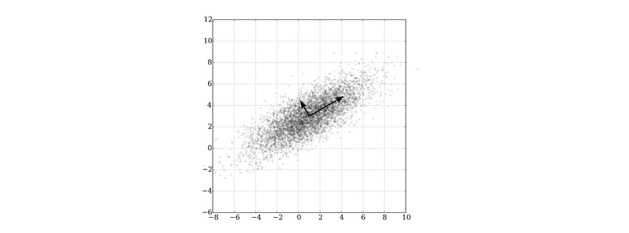 More observations in x-direction than y-direction indicates that linear regression is more “accurate” in x-direction. Therefore $\phi(a)$ in x-direction should have a tighter confidence interval. The Linear UCB model tends to pick actions in y-direction due to higher UCB and this constitute to exploration.
The formal analysis is quite involved and requires tools like Mahalanobis norm, trace rotation, and elliptical potential lemma. We will just sketch the bigger picture. Detailed derivations can be found here.
Linear Regression
Given a dataset $\{(\phi_i , r_i )\}_{i=1}^n$, data matrix $\Phi = [\phi_i]$ and reward vector $R = [r_i]$. The linear regression solves the following optimization problem:
\[\hat{\theta} = \underset{\theta \in \mathbb{R}^d}{\operatorname{argmin}} \sum_{i=1}^n ( \langle \phi_i, \theta \rangle - r_i )^2\]The analytical solution is
\[\hat{\theta} = (\Phi^\top \Phi)^{-1} \Phi^\top R\]We can analyze the error in the parameter estimation of linear regression $\hat{\theta}$:
\[\hat{\theta} - \theta^* = (\Phi^\top \Phi)^{-1} \Phi^\top Z\]where $Z$ is reward noise: $R = \Phi\theta^* + Z$.
We can also ask the question: if we compute reward $\hat{r}$ using the estimated $\hat{\theta}$, how much error does $\hat{r}$ contains:
\[\mathbb{E}_{Z \sim N(0, \sigma^2)}[\langle \phi, \hat{\theta} - \theta^* \rangle] \leq \|\phi\|_{(\Phi^\top \Phi)^{-1}} \sqrt{\sigma^2 d}\]LinUCB
Algorithm
- At round $t$, we have dataset $\{(\phi(a_i) , r_i )\}_{i=1}^{t-1}$
- Solve a ridge regression problem on dataset with L-2 regularization $\lambda$ (for more numerically stable result)
- Take action $a_t$ that have the highest UCB and observe reward $r_t$
How to pick action?
Let $\Sigma_t = \lambda I + \sum_i \phi(a_i) \phi(a_i)^\top $ be the “regularized” feature covariance at time $t$.
First construct the confidence interval of $\hat{\theta} \in \mathbb{R}^d$, where $\beta$ can be set to $\sigma^2 d$:
\[\operatorname{BALL}_t = \{ \theta: \| \theta - \hat{\theta}_t \|_{\Sigma_t} \leq \beta \}\]Then search for $a_t$ with highest UCB:
\[a_t = \underset{a \in \mathcal{A}}{\operatorname{argmax}} \underset{\theta \in \operatorname{BALL}_t}{\operatorname{max}} \langle \phi(a), \theta \rangle\]Theorem Regret bound of LinUCB
\[T \langle \phi(a^*), \theta^* \rangle - \sum_t \langle \phi(a_t), \theta^* \rangle \leq O \left(\sigma T \left(d \log( 1 + \frac{T}{\sigma^2 d} ) + \log(4/\delta) \right)\right)\]Discussion
LinUCB demonstrated that it is theoretically possible to design a algorithm with regret bound scales with $O(\sqrt{dT\log(d/\delta)})$. However, the practical value of LinUCB is limited due to:
- Complexity of hand engineering a good feature mapping $\phi$
- Linear Realizability is a strong assumption
- Computational hard to pick the action $a_t$ (two dimensional optimization problem on $\theta$ and $a$)