MCMC Diagnostics
Effective sample size (ESS)
Samples generated by MCMC method are correlated within a chain. This affect our confidence in estimation of statistics (say, posterior mean). ESS measures the information content from samples. An ESS in Markov chain Monte Carlo central limit theorem is similar to independent sample size in classic central limit theorem.
\[ESS = \frac{n}{1+2\sum_{k=1}^{\infty} \rho(k)}\]$n$ is the number of samples and $\rho(k)$ is the autocorrelation at lag $k$. If the autocorrelation is high, the sum in the denominator large, and the effective sample size is small. An autocorrelation plot can help to determine the severity of the problem. Some argue that you can “thin” the MCMC chain by discarding every k samples generated. However, you still need to allocate computational resources to generate the k samples to be discarded, which makes “thining” less useful.
Warm-up / Burn in
If we initialize the chain from a random state, the head of the chain does not follow the stationary distribution and need to be dropped. This is called “Warm-up” or “Burn in”. If you worked with low dimensional data, trace plot can be used to determine how many samples to be dropped. However this is not feasible in high dimensional problem (consider working with a Bayesian model which consists thousands of parameters; it is impossible to check all trace plots). To solve this problem, some probabilistic programming (e.g., Stan), drop first half of the samples in a by default.
Initialization
A good initialization may avoid long warm-up period in chain and save computational resources. In practice, you may use a coarse estimate (e.g., Variational Inference) to initializate MCMC. If you believe the underlying distribution is not multimodal or have high curvature regions, initializate around the centroid of a K-mean should be sufficient.
Mixing / Trace plot
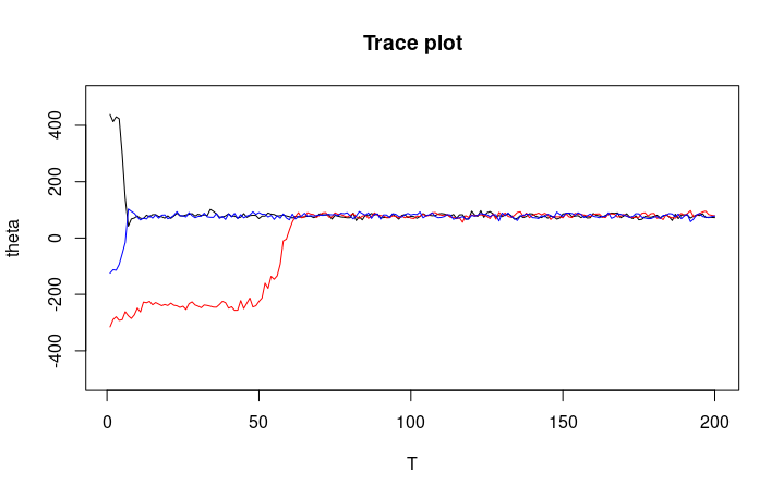
Determining if the MCMC has sufficiently explored the target distribution is hard, since the chain may stablize at a local maximium or fails to explore the tail of a distribution. In practice, we often launch multiple chains and observer their behaviors. The chain will likely started from the tail region of the distribution and slowly drift to the stationary distribution in trace plot. “Mixing” refers to the process in which markov chains converge to stationary distribution.
Trace plot also reveals userful information about the chain. For example, in Metropolis-Hastings algorithm, the trace plot can tell us if the jump proposal is too wide (too many rejections / stagnation chains) or too narrow (chains moving slowly).
If you are interested in MCMC diagnostics, you can read more in this post.