Survival Analysis
This post is mainly based on
Survival Analysis
Survival analysis is a branch of statistics which studies the time until an event occur.
Terminology
- Event
- Death of a subject in a clinical trail
- Failure of a mechanical part
- Time until a debt default
- Time-to-event: time elapsed from the beginning of the observation to
- The event occur
- Censoring
- Censoring: the survival time for that subject cannot be accurately determined
- Censoring occurred when
- The subject drops out, or is lost to follow-up
- Required data is not available
- End of study (subject survived until the end of the study, but there is no knowledge of what happened thereafter)
- Censoring occurred when
Let survival time $T$ be a random variable $T \geq 0$. $T$ induced a distribution with pdf $f(t)$ and cdf $F(t) = P (T \leq t)$. Define the survival function $S(t)$ and hazard function $h(t)$ as:
\[S(t) = P(T > t) = 1 − F(t)\] \[h(t) = \lim_{\varepsilon \rightarrow 0} \frac{P(T \in (t, t + \varepsilon] |T \geq t)}{\varepsilon}\]$S(t)$ measures the probability that the subject survives beyond time $t$. $h(t)$ measures the conditional density $f$, given the event in question has not yet occurred prior to time $t$.
Properties
- $h(t)$ is NOT the probability, but a density
- $h(t) = f (t)/S(t)$
- Hazard: risk of the event occurs
Kaplan-Meier Estimator
The Kaplan-Meier estimator is a non-parametric estimation of the survival function $S(t) = P(T > t)$. The original paper was published in 1958.
Let $\hat{S}(t)$ be the nonparametric maximum likelihood estimator of $S(t)$. If there is no censoring (the survival time can be accurately determined for all subjects), finding an estimation of the survival probability is easy:
\[\hat{S}(t) = \frac{1}{n} \sum_{i=1}^n I(T_i > t)\]However, when not all the subjects continue in the study. The censoring data adds uncertainty or can leaks information:
Given unobserved ground truth world
- $T_1, T_2, … , T_n \sim F(\cdot) = 1-S(\cdot)$, iid survival times with survivor function $S(\cdot)$
- $C_1, C_2, … , C_n$, iid censoring times
- $C_i$ is independent of $T_i$.
The observed data is $\{(U_i , \delta_i )\}_{i=1}^n$, where,
\[U_i = \min(T_i, C_i)\] \[\delta_i = I(T_i \leq C_i)\]Calculate a sequence of observed time $v_1 < v_2 < … $ from censoring time data $C_1, …, C_n$.
The Kaplan-Meier Estimator $\hat{S}(t)$ is:
\[\hat{S}(t) = \begin{cases} 1 & t < v_1 \\ \prod_{i=1}^j (1-\hat{h}_i) & v_j \leq t \leq v_{j+1} \end{cases}\]where,
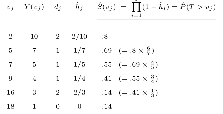
\[\hat{h}_j = \frac{d_j}{Y(v_j)}\] \[d_j = \sum_{i=1}^n \delta_i I(U_i = v_j)\] \[Y(v_j) = \sum_{i=1}^n I(U_i \geq v_j)\]$d_j$ represents number of failures/events at $v_j$ and $Y(v_j)$ represents number of “at risk” subjects at $v_j$.
Example
Given the dataset: $\{2, 2, 3^+ , 5, 5^+ , 7, 9, 16, 16, 18^+ \}$, where the number is $U$, and superscript is $\delta$, where $+$ indicate censored (outcome not determined). We can calculate the observed censoring time: $v_1 = 2, v_2 = 3, v_3 = 5, …, v_8 = 18, v_8 = 18^+$. $\hat{S}(t)$ is:
Properties
The number of failures under the failure probability $h_j$ follows a binomial distribution. The likelihood function of the data under ground truth cdf $F$ is,
\[L(F) = \prod_j h_j^{d_j} (1-h_j)^{Y(v_j) - d_j}\]The Kaplan-Meier estimator is a MLE for any cdf $F$:
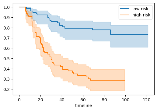
\[1 - \hat{S}(t) = \operatorname{argmax}_F L(F)\]Since $\hat{S}(t)$ is a nonparametric estimator of random variable $T$, we can also compute its Confidence Interval. In practice, the Kaplan-Meier Estimator is often visualized in plots, where x-axis is time and y-axis is survival rate. For example,
Log Rank Test
Log rank test is a two-sample nonparametric test for right censoring. The goal is to determine if there is significant difference in $\hat{S}_1(\cdot)$ and $\hat{S}_2(\cdot)$.
Due to $\hat{S}$ is a function of $t$, there are many ways that $\hat{S}_1(\cdot)$ and $\hat{S}_2(\cdot)$ can different from each other:
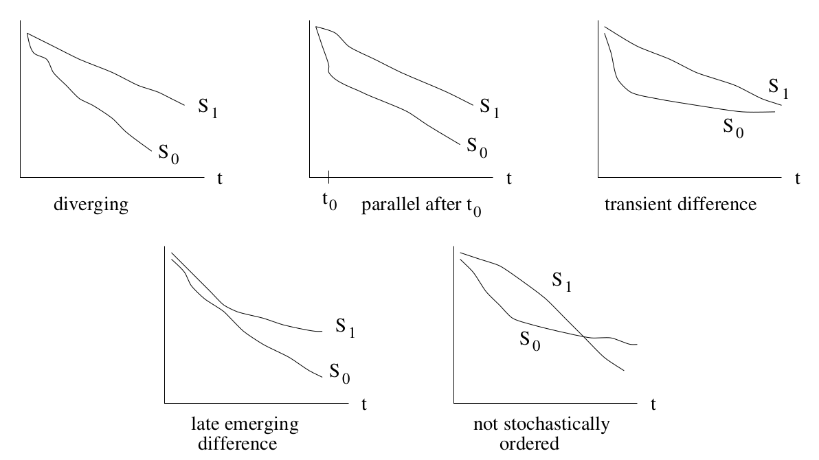
A common way to test if two samples are drawn from different distribution is to use contingency table. The idea is to compare $\hat{S}(t)$ in contingency table at different $v_1, v_2, …$. The null hypothesis $H_0$ is group 0 and group 1 fails at same rate. We can compare the observed number of failure and expected number of failure under $H_0$. Let:
- $v_1 < v_2 < …$ as defined in previous section
- $Y_i(v_j)$: # of subjects in group $i$ at risk at $v_j$
- $Y(v_j) = Y_0(v_j) + Y_1(v_j)$: Total # of subjects at risk at $v_j$
- $d_{ij}$: # of failure in group $i$ at $v_j$
- $d_j = d_{0j} + d_{1j}$: Total # of failures at $v_j$
Then,
- $O_j = d_{1j}$: observed # of failures in group 1
- $E_j = d_j \frac{Y_1(v_j)}{Y(v_j)}$: expected # of failures in group 1
- $V_j = \frac{Y_0(v_j)Y_1(v_j)d_j(Y(v_j)-d_j)}{Y(v_j)^2(Y(v_j)-1)}$: variance of the observed # of failures
Under $H_0$, the log rank test statistics is:
\[Z = \frac{\sum_j (O_j - E_j)}{\sqrt{\sum_j V_j}} \sim \mathcal{N}(0,1)\]Properties
- The power of the test depends on the number of observed failures rather than the sample sizes
Proportional-Hazards Model
The Proportional-Hazards (PH) Model is also called the Cox Model. While log rank test can only be used to analyze survival function of 2 groups, PH model can be used to analyze the effect of multiple risk factors on survival time.
The survival model can be viewed as 2 parts:
- Baseline hazard function: $\lambda_0(t)$
- Effect parameters: $\exp( X \cdot \beta)$
The hazard function for PH model is defined as:
\[\lambda(t|X_i) = \lambda_0(t)\exp(X_i \cdot \beta)\]If features $j$ is not statistical significant, $\beta_j = 0$ and $\exp(\beta_j) = 1$. This indicates that features $j$ has little effect on survival time. We can check the p-value of $\beta_j$ to determine if features $j$ is statistical significant to survival time.
“Proportional” Hazard
The term Proportional comes from the fact that effect of feature is multiplicative:
Given $\lambda(t |x) = \lambda_0(t) \exp(\beta x)$, we have,
\[\lambda(t|x+1) = \lambda_0(t) \exp(\beta (x + 1)) = \lambda_0(t) \exp(\beta x) \exp(\beta)\]Hence,
\[\frac{\lambda(t|x+1)}{\lambda(t|x)} = \exp(\beta)\]The effect of increasing $x$ be one unit is always fixed, or the effect is “proportional.”