Copula
I encountered Copula at Dr. Gunter Meissner’s topic course on CDO pricing.
Problem setup
Consider a portfolio consisting $d$ bonds. Each bond can default and let the default year for bond $i$ be a random variable $X_i$. Then each $X_i$ induced a probability distribution $P_i(X_i = x_i)$ where $x_i$ is a future date, say year $x_i$. To price this portfolio, we need to consider the joint $p(x_1, x_2, … x_d)$ and calculate an expectation:
\[\mathbb{E}[\text{loss}] = \sum_{x_1, ..., x_d} \text{loss}(x_1, ..., x_d) p(x_1, ..., x_d)\]The main problem is $X_i$ are not independent: default in one or two bonds may be caused by some random events; however, in recession, most issuers will face cash flow problems and default events are likely highly correlated.
When I think about this problem, I realized that:
- Most my training in probability concerns with finding marginals from the joint. In case of getting the joint from marginals, we usually assume independence.
- I did not use a lot of multivariate distributions in practice (distributions that I can call out names are: Multinomial distribution, Multivariate gaussian, Multivariate t-distribution and Wishart distribution)
Definition
Loosely speaking, copula is an interesting tool that map multiple marginal distribution to a joint distribution. Consider random variable $X_1, X_2, .., X_d$ and their marginal cumulative distribution function (CDF) $F_i(X_i)$. From Probability integral transform, we know that each marginal $F_i(X_i)$ is uniformly distributed on the interval $[0, 1]$. Let $U_i$ be a random variable s.t., $U_i = F_i(X_i)$. We now have $U_1, U_2, …, U_d$ each uniformly distributed.
The copula of $( X_1 , X_2 , … , X_d )$ is defined as the joint cumulative distribution function of $( U_1 , U_2 , … , U_d )$:
\[\Pr[U_1\leq u_1,U_2\leq u_2,\dots ,U_d\leq u_d] = C(u_1,u_2,\dots ,u_d) = C(F_1(x_1), ... , F_d(x_d))\]According to the formal definition, Copula is just the joint $P(u_1 , u_2 , … , u_d )$: $[0,1]^d \rightarrow [0,1]$.
Looking at this definition, there are two takeaways:
- Copula $C$ induces the dependence structure between $(X_{1},X_{2},\dots ,X_d)$ by $U_i$
- Information is linked via
- Joint of $U_i: C(u_{1},u_{2},\dots ,u_{d})$
- CDF $F_i(x_i)$
- Inverse CDF $F^{-1}_i(u_i)$ (The distribution of $F^{-1}_i(u_i)$, where $u_i \sim \text{unif}[0,1]$ is the marginal of $X_i$)
- Information is linked via
- We can “fit a model” from data
- Assume different joint distribution $C$ and estimate the parameter $\theta_C$
- Assume different marginal distribution $F_i$ and estimate the parameter $\theta_i$
Considering the Inverse CDF $F^{-1}_i(u_i)$, if we reverse the above steps, we can get a sampling tool for the multivariate probability distributions.
\[(X_1, X_2, ... , X_d) = ( F_1^{-1}(U_1), F_2^{-1}(U_2), ... , F_d^{-1}(U_d))\]where $(U_1, U_2, …, U_d) \sim c(u_1,u_2,\dots ,u_d)$
And $c(u_1,u_2,\dots ,u_d)$ is the PDF of $C(u_1,u_2,\dots ,u_d)$.
Sklar’s theorem
Sklar’s theorem deals with the existence and uniqueness of copula. It states that every multivariate cumulative distribution function $H(x_1, …, x_d) = P[X_1\leq x_1,\dots ,X_d\leq x_d]$ can be expressed in its marginals $F_i(x_i)=\Pr[X_i\leq x_i]$ and a copula $C$.
\[H(x_1, ... , x_d) = C(F_1(x_1), . . . , F_d(x_d))\]Moreover, its PDF $h(x)$ has the form
\[h(x_1, ..., x_d) = c(F_1(x_1),\dots ,F_d(x_d)) \cdot f_1(x_1) \cdot \dots \cdot f_d(x_d)\]where $c$ is the PDF of $C$ and $f_i$ is the PDF of $F_i$.
When the marginals $F_{i}$ are continuous, then inverse CDF exist $x_i = F^{-1}_i(u_i)$,
\[\begin{align} H(x_1, ... , x_d) &= C(F_1(x_1), ... , F_d(x_d))\\ H(F_1^{-1}(u_i), ... , F_d^{-1}(u_d)) &= C(u_1, ... , u_d)\\ \end{align}\]Gaussian copula
Recall the above result: $C(u_1,u_2,\dots ,u_d) = H(F_1^{-1}(u_i), … , F_d^{-1}(u_d))$, where $F_i^{-1}$ is inverse CDF. Taking $H$ as multivariate Gaussian distribution, we have,
\[\begin{align} C_{R}^{\text{Gauss}}(u) &= \Phi _{R}\left(\Phi ^{-1}(u_{1}),\dots ,\Phi ^{-1}(u_{d})\right)\\ &=\frac{1}{\sqrt{\det {\Sigma}}} \exp \left(-{\frac {1}{2}}{\begin{pmatrix}\Phi ^{-1}(u_{1})\\\vdots \\\Phi ^{-1}(u_{d})\end{pmatrix}}^{T}\cdot \left(\Sigma^{-1}-I\right)\cdot {\begin{pmatrix}\Phi ^{-1}(u_{1})\\\vdots \\\Phi ^{-1}(u_{d})\end{pmatrix}}\right) \end{align}\]where $\Sigma$ is the covariance matrix and $\Phi ^{-1}: [0,1] \rightarrow [-\infty, \infty]$ is inverse cumulative distribution function (or quantile function) of gaussian distribution.
Going back to the context of CDO pricing, consider our portfolio contains only B rated bond. We can compute a default probability table for those B rated bond from historical data. If we are interested in two bonds default in years 3, the marginal cumulative default probability (i.e., CDF for $x_i$) is 21.03%. Then, compute the inverse CDF $\Phi^{-1}(0.2103)$. Given the default correlation matrix $\Sigma$, we can compute joint probability using the above formula.
Obviously, B rated bond from one issuer is different from B rated bond from another issuer so we may not have enough data to estimate $\Sigma$. Inverting $\Sigma$ could also be unstable. According to Dr. Meissner, trader often use a simplified model called One-Factor Gaussian Copula Model (OFGC) in practice, which is much cheaper to compute and generally delivers good performance.
In terms of evaluation of tail risk, student-t copula and Gumbel copula are better choices.
Archimedean copulas
Let’s view the “get joint from marginal” problem from a different perspective: consider we have two event $A$ and $B$. $P(A) = 0.7$ and $P(B)=0.8$. Ideally, we want to perform arithmetic operations directly on marginals $P(A), P(B)$ to get the joint $P(A,B)$. Let’s say we perform $P(A) + P(B) = 1.5$. Obviously, the above calculation is not valid ($1.5 > 1$). One way of interpretation is that the above calculation fails due to $1.5$ is out of range $[0,1]$. If we can find a function that maps the $1.5$ back to $[0,1]$, can we find a proper way to compute joint distribution $P(A,B)$?
The idea of Archimedean copulas is as follow: suppose we have
- A generator function $\phi(x): [0,1] \rightarrow [0, \infty]$ where $\phi(1) = 0$ and $\phi(0) = \infty$
- $\phi(x)$ has an inverse $\phi^{-1}(x)$ where $\phi^{-1}(\phi(F(x))) = F(x)$
We can compute the joint as $P(x_1, …, x_d) = \phi^{-1}\left[\sum_{i=1}^d \phi( F(x_i) )\right]$, where we first map $x$ to $[0, \infty]$ using $\phi$, then map $\phi(x)$ back to $[0,1]$ using $\phi^{-1}$ for a valid probability.
For example, Let $\phi(x)=\ln(x)$ and $\phi^{-1}(x) = e^{-x}$. Then,
\[\begin{align} P(A \cap B) &= e^{-[-\ln(P(A)) -\ln(P(A))]} \\ &= e^{-(0.22314+0.35667)}\\ &= 0.56000 \end{align}\]Observe the result of the above calculation is equal to $P(A) \cdot P(B)$. This is not a coincidence as the generator function implies the Independence copula.
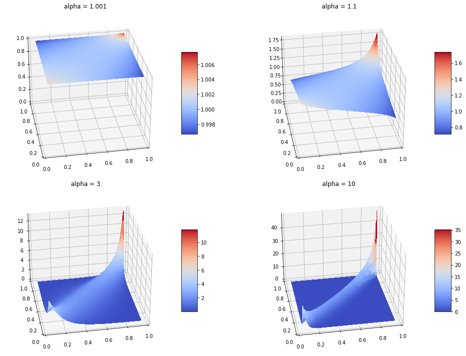
Gumbel copula
Gumbel Copula takes a different generator function
- $\phi(x) = (-\ln x)^\alpha$
- $\phi^{-1}(x) = e^{-x^\frac{1}{\alpha}}$
Parameter $\alpha$ can be estimated by Kendall’s $\tau$.
Gumbel copula has upper tail dependency. This means correlation $\rho \uparrow$ as $x$ takes on extremely positive values, which is shown in the density plot below:
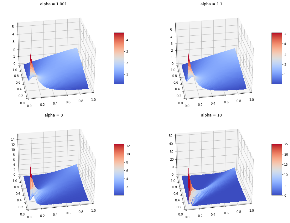
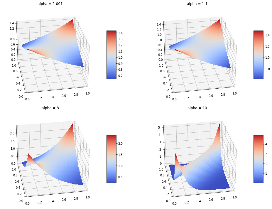
Clayton copula and Frank copula
There are other Archimedean copulas which uses different generator functions. For example: Clayton Copula and Frank Copula.
Clayton Copula has lower tail dependency, which is shown in the density plot below:
Frank Copula has both upper and lower tail dependency, which is shown in the density plot below:
Script for generating the above plots can be found here
Estimation of copula
Now we have the model (copula) in our toolbox, we need a way to fit the model to the data. If you are interested in this topic, take a look at Yen-Chi Chen’s Note. Chen mentioned three ways for parameter estimation: parametric approach, semi-parametric approach and nonparametric approach.
Let $\theta_i$ be the parameters for $F_i$ and $\theta_c$ be the paramters for the copula. In the parametric approach, we write down the full log-likelihood $\mathcal{l}_c(\theta_i, \theta_c |x)$ (including both copula density and marginal) and perform a MLE on $\mathcal{l}_c(\theta_i, \theta_c |x)$.
In semi-parametric approach, we first estimate parameters $\mathcal{l}_c(\theta_i |x)$ for the marginals $F_i$ then estimate the parameter for the copula $\mathcal{l}_c(\theta_c |x, F_i)$.
In Nonparametric approach, we still use the two-step method similar to semi-parametric approach, but the parameter for the copula is estimated by a nonparametric density estimator, rather than log-likelihood $\mathcal{l}_c(\theta|x, F_i)$.