Legendre Memory Units

This post is mainly based on

Legendre Memory Units / LMU

LMU
- Memory cells $m(t)$ are mathematically derived to remember the history $u(t)$
- $m(t)$ remember the history $u(t)$ by projecting $u(t)$ onto orthogonal polynomials basis
Results
- Outperforms equivalently-sized LSTMs on
  - Chaotic time-series prediction
  - pMNIST
- Improves memory capacity by two orders of magnitude (100,000 time-steps)
- Use few internal state-variables to learn complex functions
- Significantly reduces training and inference time

LMU Architecture

Input: $x$
LMU Layer
- Memory cell $m$
  - Memorize input history
  - Input: $u_t = e_x \cdot x_t + e_h \cdot h_{t-1} + e_m \cdot m_{t-1}$
  - $u_t \in \mathbb{R}$: encoded history to memorize
  - $e_x, e_h, e_m$: learned encoding vectors
  - $\bar{A}, \bar{B}$: matrices output from ODE solver or fixed (see below)
- Hidden cell $h$:
  - Apply non-linear transformation
  - $h_t = f(W_x x_t + W_h h_{t-1} + W_m m_t)$
  - $f$: non-linear activation
  - $W_x, W_h, W_m$: learned projection matrices
Output: $h$

arch

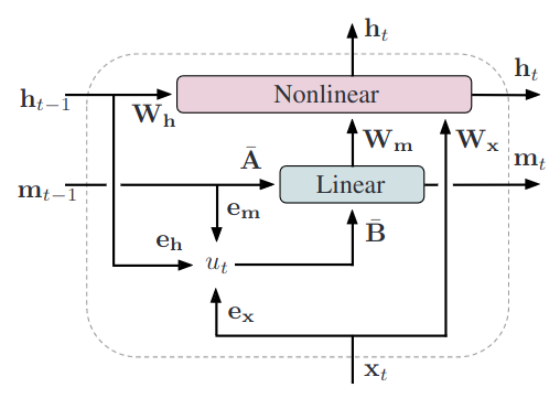
Time-unrolled LMU layer. An n-dimensional state-vector ($h_t$) is dynamically coupled with a d-dimensional memory vector ($m_t$). The memory represents a sliding window of $u_t$, projected onto the first d Legendre polynomials.

Memory cell $m(t)$

Given a continuous-time input signal, $u(t) \in \mathbb{R}$, $m$ is designed to memoize history of $u(t)$ within a sliding window $[t-\theta, t]$, where $\theta \in \mathbb{R}$ is the length of history.

LMU attempt to memoize the history of $u(t)$ by storing a d-dimensional state-vector $m(t)$. $m(t)$ is coefficients of a set of orthogonal polynomials basis $f_1, f_2, … f_d$. You can approximate the history of $u(t)$ within the sliding window by summing up the basis with their coefficients:

\[u(t) \approx m_1(t) f_1(t) + m_2(t) f_2(t) + ... + m_d(t) f_d(t)\]

The higher the order $d$, the high frequency $u(t)$ you can approximate. Legendre polynomials are chosen as the orthogonal polynomials basis.

legendre-poly

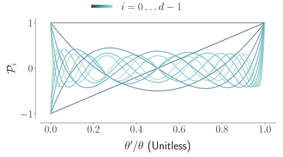
Shifted Legendre polynomials (d = 12). The memory of the LMU represents the entire sliding window of input history as a linear combination of these scale-invariant polynomials. Increasing the number of dimensions supports the storage of higher-frequency inputs relative to the time-scale.

The paper stated that the $u(t)$ history is best approximated by $d$ coupled ordinary differential equations (ODEs):

\[\theta \dot{m}(t) = Am(t) + Bu(t)\]

The matrix $A$ and $B$ are derived through Pade approximants:

\[A = [a_{ij}] \in \mathbb{R}^{d \times d}, \quad a_{ij} = \begin{cases} -1 & \text{if } i < j, \\ (-1)^{j+i+1} & \text{if } i \geq j \end{cases}\] \[B = [b_i] \in \mathbb{R}^{d \times 1}, \quad b_i = (2i + 1)(-1)^i, \quad i,j \in [0, d-1]\]

And the Pade approximants corresponds to shifted Legendre polynomials as their temporal basis functions, described in Section 6.1.3 of the Dynamical Systems in Spiking Neuromorphic Hardware thesis.

Given the above theoretical results, the time-delayed u(t) can be reconstructed as:

\[u(t-\theta') \approx \sum_{i=0}^{d-1} \mathcal{P}_i (\frac{\theta'}{\theta}) m_i(t)\]

where $ 0 \leq \theta’ \leq \theta $ and $\mathcal{P}_i$ is the i-th shifted Legendre polynomial.

Discretization

Further, to map the continuous ODE to discrete time steps in a recurrent neural network, we have the below Discretization:

\[m_t = \bar{A}m_{t−1} + \bar{B}u_t\]

The matrix $\bar{A}$ and $\bar{B}$ are provided by the ODE solver for some time-step $\Delta t$ relative to the window length $\theta$. i.e., As you change $\Delta t / \theta$, $\bar{A}$ and $\bar{B}$ will also change.

However, if $\Delta t / \theta$ is sufficiently small, the non-linearity of the ODE is ignorable, hence we can directly obtain $\bar{A}$ and $\bar{B}$ using Euler’s method:

\[\bar{A} = (\Delta t / \theta) A + I\] \[\bar{B} = (\Delta t / \theta) B\]

Personal thought: since this paper does not provide a comprehensive description of of how memorizing history, delay operator, ODEs, Pade approximants and Legendre polynomials connect together, and since these areas are outside my expertise, I’m taking the paper’s words at their face value without really understanding their internal links. Should you identify any errors or wish to share your thoughts, please feel reach out.

Experiments

Initialization
- $\bar{A}$ and $\bar{B}$: using Pade approximants $A,B$ and zero-order hold (ZOH)
- $\theta$: prior knowledge of the task
- $W_m$: the authors mentioned using the $u(t-\theta’)$ equation to initialize without further details
- $e_m = 0$, to ensure stability
- $W_x, W_h$: Xavier normal
- $e_x, e_h$: LeCun uniform
- $f$: $\tanh$
Optimization
- $\bar{A}$, $\bar{B}$ and $\theta$ are not optimized

Copy Memory Task

Task: maintain $T$ values in memory for large values of $T$ relative to the size of the network
Refer to paper’s Section 3.1 for details on Model Complexity and Memory Cell Isolation

copy

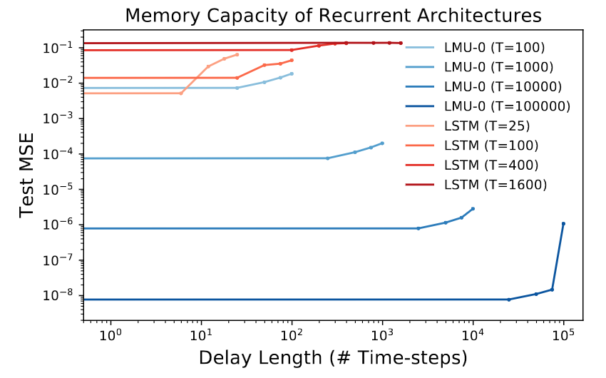
Comparing LSTMs to LMUs while scaling the number of time-steps between the input and output. Each curve corresponds to a model trained at a different window length, $T$, and evaluated at 5 different delay lengths across the window. The LMU successfully persists information across 105 time-steps using only 105 internal state-variables, and without any training.

pMNIST

Outperforms SOTA RNN models
LMU Model size
- Hidden units: $n = 212$
- Memory: $d = 256$
- Sliding window: $\theta = 784$
- Total $n + d = 468$ variables in memory between time-steps, which is less than $28^2 = 784$ pixels
- Smaller than SOTA model (NRU)
Convergence
- LMU: 10 epochs
- NRU: 100 epochs

pmnist

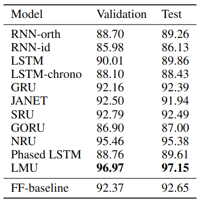
Validation and test set accuracy for psMNIST.

Mackey-Glass Prediction

Task: chaotic dynamical system, predict 15 time-steps into future
- Hard: due to butterfly effect
- Any perturbations to the estimate of the underlying state diverge exponentially over time
LMU Model size
- 4 layers, ~18k parameter
- $n = 49$, $d = 4$, $\theta = 4$

chaotic

Mackey-Glass results.