RNNs for Irregularly Spaced Time Series
This post is mainly based on
- Modeling Missing Data in Clinical Time Series with RNNs, 2016
- GRU-D: Recurrent Neural Networks for Multivariate Time Series with Missing Values, 2016
- CT-GRU: Discrete-Event Continuous-Time Recurrent Nets, 2017
Irregularly Space Time Series
- Real-world time-series observations are recorded irregularly, with measurement frequency varying between data sources, variables and over time
- Simple Imputation: fix-width time steps + imputation + indicator variable
- GRU-D: variable-width time steps + time interval width + decay
- CT-GRU: decomposition of hidden state decaying at different rates
Simple Imputation
- Strategy: Group observations into a sequence with discrete, fixed-width time steps
- Data processing: Indicator Variable + Imputation
- Performance: significantly outperforms Linear Regression / MLP / Engineered features
Missing Values
- Missing values are not missing at random
- The pattern of recorded measurements could contain potential information about the state of the data source
- For example, in clinical setting, the fact that some lab values are measured more often than other may implies state of patients
- Heuristic or unsupervised imputation ignores the information carried in the missingness itself
Treatment
- Indicator Variable
- if $x^{(t)}_i$ is missing, set $m^{(t)}_i = 1$
- Imputation
- Zero imputation: $x^{(t)}_i = 0$ if missing variable $i$ at time step $t$
- Forward-filling: $x^{(t)}_i = x^{(t’)}_i$ for previous recorded time step $t’$
- If no previous measurement available, use training data median
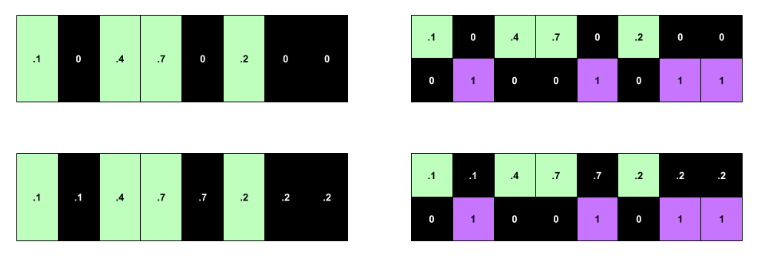
Top left: no imputation or indicators. Bottom left: imputation absent indicators. Top right: indicators but no imputation. Bottom right: indicators and imputation. Time flows from left to right.
Experiments
- Data
- Irregularly spaced measurements of 13 variables in clinical dataset
- Combine multiple measurements of the same variable within the same hour window by taking their mean
- Scale each variable to the [0, 1] interval, using expert-defined ranges
- Model: LSTM
- Layer = 2
- Dim = 128
- Non-recurrent dropout = 0.5
- L-2 weight decay = $10^{−6}$
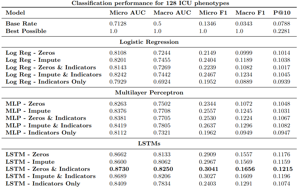
Performance on aggregate metrics for logistic regression (Log Reg), MLP, and LSTM classifiers with and without imputation and missing data indicators.
Analysis of Result
- RNN out-performs Hand-Engineered Features
- Missing pattern contains information
- See:
LSTM - Indicators Only
- See:
- Even without indicators, the RNN might learn to recognize filled-in vs real values
- For forward-filling, the RNN could learn to recognize exact repeats
- For zero-filling, the RNN could recognize that values set to exactly 0 were likely missing measurements
- See:
LSTM - ZerosandLSTM - Impute
GRU-D
- Handle variable-width time steps with missing values
- Missing values: imputation + indicator variable
- Variable-width time steps: absolute time + $\Delta$ time
- Outperforms SOTA on MIMIC-III, PhysioNet mortality prediction
Treatment
- Data pre-processing / added dimensions
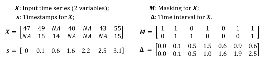
An example of measurement vectors $x_t$, time stamps $s_t$, masking $m_t$, and time interval $\delta_t$.
GRU-D
- GRU-D: GRU with trainable decay
- Influence of the input variables will fade away over time if the variable has been missing for a while
- Decay
- Input decay rate: $\gamma_t$
- Hidden state decay rate: $\gamma_h$
Input decay
\[\gamma_t = \exp \{ -\max(0, W_\gamma \delta_t + b_\gamma) \}\]where $W_\gamma, b_\gamma$ are trainable and $W_\gamma$ constrain to be diagonal (decay rate of each variable independent from the others).
Input decay is directly applied to forward imputed missing value to decay it over time toward the empirical mean
\[\gamma_t^d x_{t'}^d + (1-\gamma_t^d)\tilde{x}^d\]where,
- $d$: dimension number
- $x_{t’}^d$: last observation of the d-th variable
- $\tilde{x}^d$: empirical mean of the d-th variable
Hidden state decay
\[h_{t-1} \leftarrow \gamma_h \odot h_{h-1}\]where $W_\gamma$ is not constrain to be diagonal
GRU-D
\[z_t = \sigma(W_z x_t + U_z h_{t-1} + V_z m_t + b_z)\] \[r_t = \sigma(W_r x_t + U_r h_{t-1} + V_r m_t + b_r)\] \[\tilde{h}_t = \tanh(W x_t + U (r_t \odot h_{t-1}) + V m_t + b)\] \[h_t = (1 - z_t) \odot h_{t-1} + z_t \odot \tilde{h}_t\]where $\odot$ is element-wise multiplication
GRU for Reference
\[z_t = \sigma(W_z x_t + U_z h_{t-1} + b_z)\] \[r_t = \sigma(W_r x_t + U_r h_{t-1} + b_r)\] \[\tilde{h}_t = \tanh(W x_t + U (r_t \odot h_{t-1}) + b)\] \[h_t = (1 - z_t) \odot h_{t-1} + z_t \odot \tilde{h}_t\]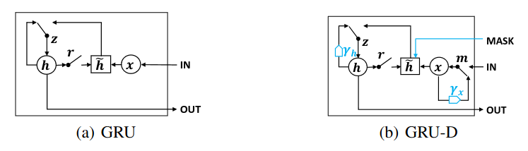
Experiments
- Datasets
- MIMIC-III: ICD-9 20 tasks
- PhysioNet: All 4 tasks
- Baseline: indicator variable ($m_t$) + mean/forward imputation
- Adding $\delta_t$ improves performance (GRU-simple)
- Adding learned decay parameter further improves performance (GRU-D)
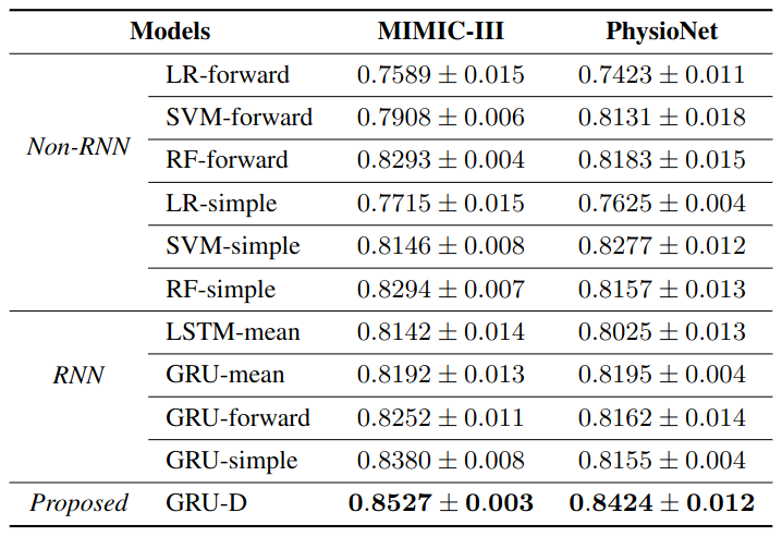
Model performances measured by AUC score (mean ± std) for mortality prediction.
Ablation
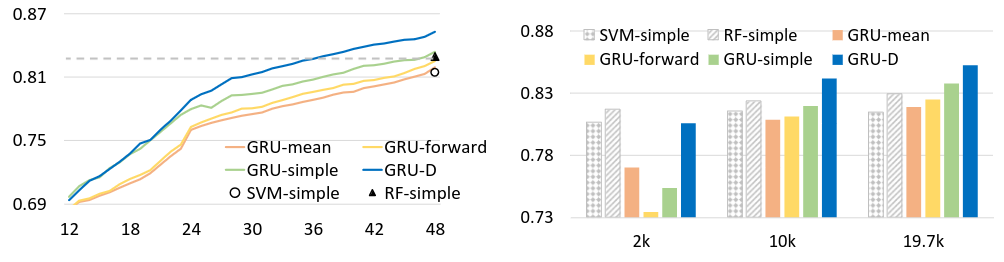
Left: GRU-D performance continued to increased when given longer historical data. x-axis, # of hours after admission; y-axis, AUC score; Dash line, RF-simple results for 48 hours.
Right: GRU-D scaled better with more training data. x-axis, subsampled dataset size; y-axis, AUC score.
CT-GRU / Hidden State Decomposition
- Impact of event could be short-lived or long-lasting
- Decompose hidden state $h$ into memory-decaying at different rate
- Each decaying rate is called a trace
- Store event in different traces
- Results: fails to outperform benchmark
Background
- Problems with GRU
- Sequences may have different structure at different scales
- GRU has too much flexibility / no inductive bias on hidden state decay
- Goal: Add a temporal inductive bias to RNN (similar to spatial inductive bias of CNN)
- Continuous-time GRU (CT-GRU)
- Endow each hidden unit with multiple memory traces that span a range of time scales
- Define future state $h$ as differential equation: $dh/dt = -h/\tau$
- Hence, $h(t) = e^{-t/\tau} h(0)$
- Time-scale $\tau$ is defined as the time for the state to decay to a proportion $e^{−1} = 0.37$ of its initial level
Suppose impact of event decay at ground truth rate $\tau^s_k$
- $s$: “storage”
- $k$: time step
Fixed set of M traces with log-linear spaced time scales: $\tilde{T} = { \tau_1, \tau_2, …, \tau_M }$ Approximate true $\tau^s_k$ by a mixture of traces from $\tilde{T}$
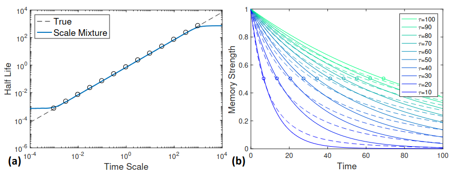
(a) Half life for a range of time scales: true value (dashed black line) and mixture approximation (blue line). (b) Decay curves for time scales $\tau \in [10, 100]$ (solid lines) and the mixture approximation (dashed lines).
CT-GRU
- Refer to paper’s Section 2.2
Experiments
- Baseline model
- GRU
- GRU with $\Delta t$ (add time-lag between current event and previous event as input)
- CT-GRU fails to outperform benchmark
- CT-GRU performs no better than the GRU with $\Delta t$ on Synthetic / Real world dataset
- The author suggest that: Although CT-GRU and GRU enforce different degree of flexibility, but perhaps the space of solutions they can encode is roughly the same