Vision Transformer (ViT)

This post is mainly based on

• ViT: An Image is Worth 16x16 Words: Transformers for Image Recognition at Scale, ICLR 2021
• DeiT: Training data-efficient image transformers & distillation through attention, PMLR 2021

ViT

• Reliance on CNNs is not necessary / pure transformer on image patches performs well
• Pre-trained on large amounts of data (JFT-300M or ImageNet-21k)
• Fine-tuned model is SOTA competitive on small benchmarks (ImageNet, CIFAR-100, VTAB)

Background

• Previous works
  • Some works try to combining CNN with self-attention
  • Other works remove CNN, but not yet been scaled effectively on modern hardware accelerators due to the use of specialized attention patterns
  • Classic ResNetlike architectures are still SOTA
• ViT
  • Split an image into patches and provide the sequence of linear embeddings of these patches
• On mid-sized datasets (ImageNet without strong regularization)
  • ViT performance lag behind SOTA model of comparable size
  • Possible reason: Transformers lack some of the inductive biases inherent to CNNs, such as translation equivariance and locality
• On larger datasets (14M-300M images)
  • Large scale training trumps inductive bias and model performance is SOTA competitive

Architecture

• Reshape
  • From: $x \in R^{H \times W \times C}$
  • To: $x_p \in R^{N \times (P^2 \cdot C)}$
  • $(H,W)$: image original resolution
  • $(P,P)$: resolution for each image patch
  • $N = HW/P^2$: effective input sequence length
• Linear Projection / Patch Embedding
  • Flatten each patch: $P \times P \times C \rightarrow P^2 \cdot C$
  • $x_p = [x_p^1, x_p^2, …., x_p^N]$
  • Map flattened patch to transformer dimension $D$: $x_p^i E$
  • $E$ is linear projection matrix
• Special Token
  • Append 1 Learnable embedding at the beginning of the sequence, similar to [class] token
  • $y$: corresponding output representation at the top of transformer
• Classification Head
  • Take $y$ and output class
  • Pre-training: MLP with 1 hidden layer
  • Fine-tuning: Linear layer
• Position Embedding
  • 1D
  • No significant performance gains from 2D embedding

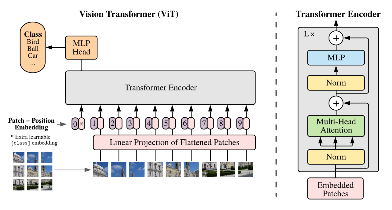
Model Architecture. Left: Image is split into fixed-size patches. Then each patch is applied linear mapping and add position embeddings. The resulting sequence of vectors are feed to a standard Transformer encoder. “0” and “*” are position 0 and learnable classification token.

ViT vs CNN

• CNN
  • All conv layers have local inductive bias and are translationally invariant
• ViT
  • Only MLP have local inductive bias and are translationally invariant
  • All transformer blocks are global
  • Positional embedding inject location information into each patch, hence transformer blocks are not translationally invariant

Resolution

• ViT can accept image with different resolution
• Patch size and linear project remains the same, but sequence length increase
• The pre-trained position embeddings may no longer be meaningful
  • Requires 2D interpolation of the pre-trained position embeddings, according to their location in the original image

Experiments

• Datasets
  • Pre-training
    • ImageNet-1k: 1k classes and 1.3M images
    • ImageNet-21k: 21k classes and 14M images
    • JFT-300M: 18k classes and 303M high-resolution images
  • Fine-tuning / Benchmark tasks
    • ImageNet original validation labels
    • ImageNet cleaned-up ReaL labels
    • CIFAR-10/100
    • Oxford-IIIT Pets
    • Oxford Flowers-102
    • 19-task VTAB classification suite: low-data transfer to diverse tasks
• Models
  • ViT-B: BERT Base architecture, 86M params
  • ViT-L: BERT Large architecture, 307M params
  • ViT-H: “Huge” model, 32 Layers, 1280 hidden size, 632M params
  • ViT-L/16: “Large” variant with 16 x 16 input patch size
• CNN Baseline: ResNet / BiT
  • Switch from BatchNorm to GroupNorm
  • Standardized convolutions
  • These changes improves model transfer

Results

• ViT-L/16, JFT-300M
  • Outperforms BiT-L on all tasks
  • Requires substantially less computational resources to train
• ViT-H/14, JFT-300M
  • Further improves the performance
  • Especially on ImageNet, CIFAR-100, and the VTAB suite

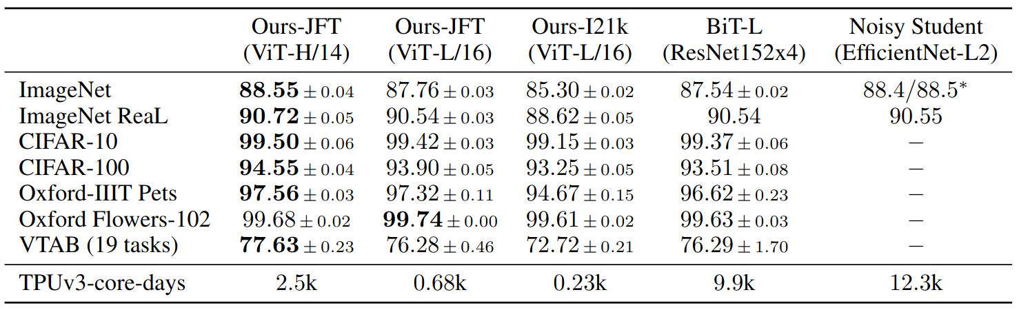
Comparison with SOTA on popular image classification benchmarks, averaged over three fine-tuning run. ViT models pre-trained on the JFT-300M dataset outperform ResNet-based baselines on all datasets, while taking substantially less computational resources to pre-train.

Ablation: Model vs Pre-training Size

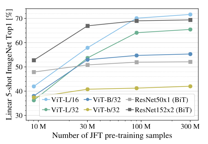
ResNets perform better with smaller pre-training datasets but plateau sooner than ViT, which performs better with larger pre-training. ViT-b is ViT-B with all hidden dimensions halved.

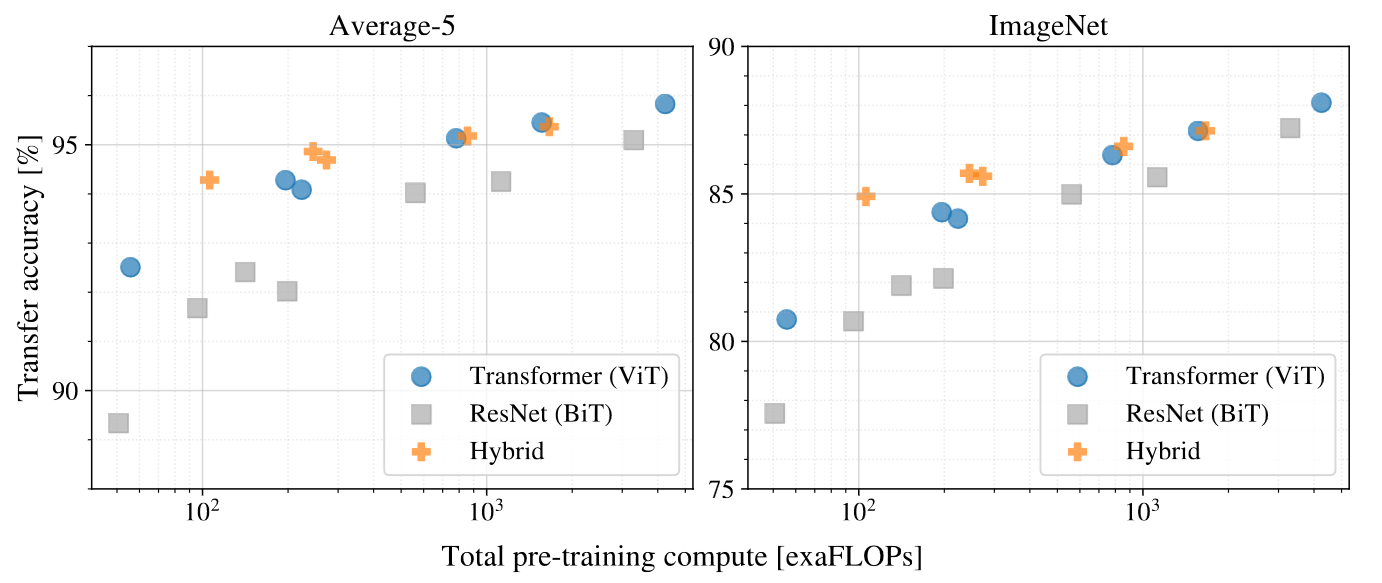
Performance versus pre-training compute. ViT uses approximately 2-4x less compute to attain the same performance.

Attention

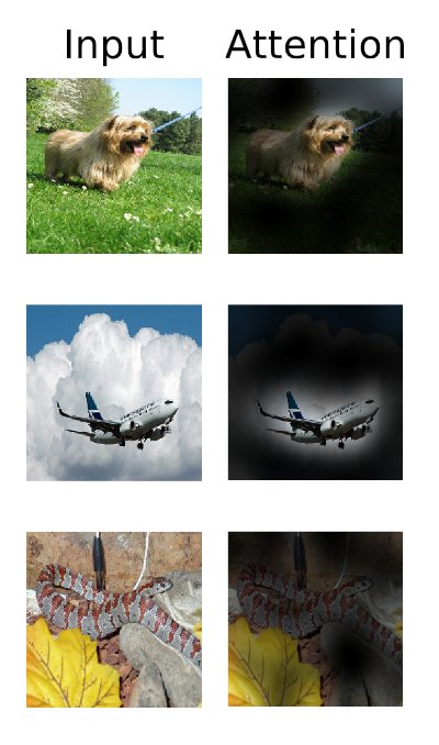
Attention from the output token to the input space, quantified by Attention Rollout. see Appendix D.8

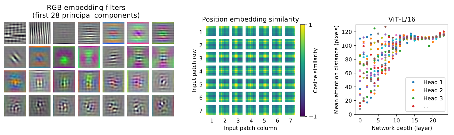
Left: Filters of the initial linear embedding of RGB values of ViT-L/32. Center: Similarity of position embeddings of ViT-L/32. Right: Size of attended area by head and network depth. Each dot shows the mean attention distance across images for one of 16 heads at one layer. Attention distance: see Appendix D.7.

Limitations

• Requires label: self-supervised pre-training still underperforms supervised pre-training

DeiT

• Extensive ablation study on ViT training
  • 86M params ViT trained on Imagenet-1k, with a single computer in <3 days
  • ImageNet top-1 accuracy: vanilla=83.1%, distillation=85.2% (SOTA competitive)
• Distillation: Teacher-student strategy

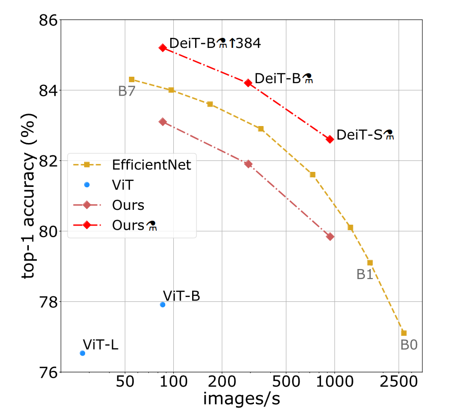
Throughput vs accuracy on Imagenet. Throughput is measured on 1 V100 GPU. DeiT-B and VIT-B has almost identical architecture, but DeiT-B is trained/optimized with a strategy for smaller dataset. The $m$ symbol represent distillation.

Background

• ViT paper: transformers “do not generalize well when trained on insufficient amounts of data”
• DeiT paper: generalization is possible with a medium size dataset, with correct hyper-parameters and repeated augmentation
• Knowledge Distillation (KD)
  • Training of a student model leverages “soft” labels coming from a strong teacher network
  • Hard label: class label
  • Soft label: softmax vector over class label
  • KD can be regarded as a form of compression of the teacher model
  • KD can transfer inductive biases in a soft way

Overview

• DeiT-S and DeiT-Ti have fewer parameters and can be seen as the counterpart of ResNet-50 and ResNet-18
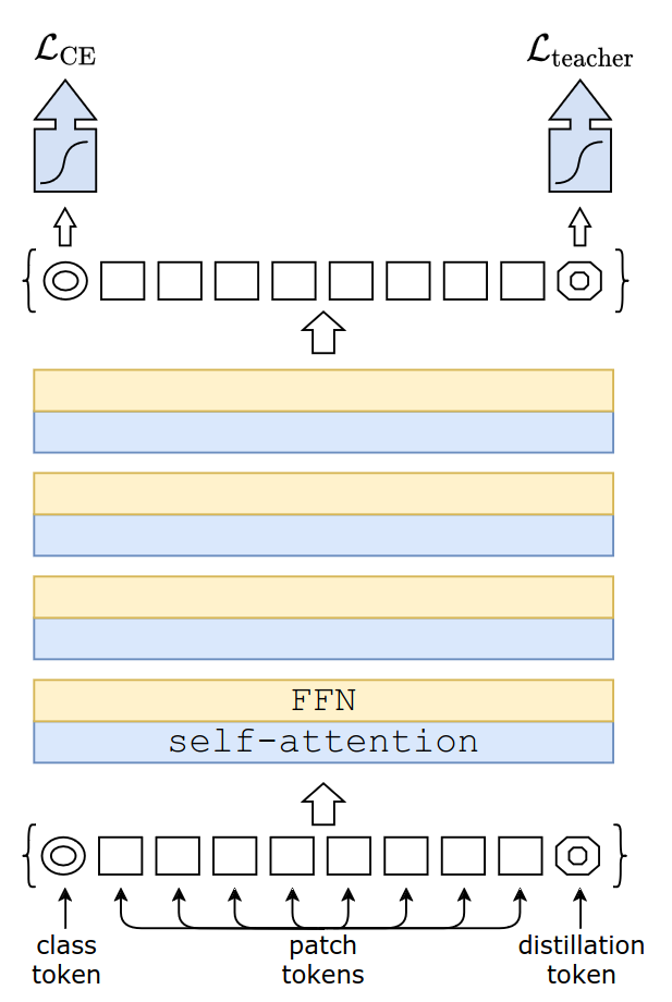
• The new distillation procedure is based on a distillation token, which plays the same role as the class token, except that it aims at reproducing the label estimated by the teacher
• With our distillation, image transformers learn more from a convnet than from another transformer with comparable performance
• SOTA competitive on transfer learning: CIFAR-10, CIFAR-100, Oxford-102 flowers, Stanford Cars and iNaturalist-18/19

Distillation through attention

• Requirement: access to a teacher model
• Ablations
  • Trade-off between accuracy and image throughput
  • Hard distillation vs soft distillation
  • Classical distillation vs the distillation token
• Soft distillation
  • Minimize the KL-divergence of the softmax between teacher and student model
  • $L = (1-\lambda)L_{CE}(\psi(Z_s),y) + \lambda \tau^2 KL(\psi(Z_s/\tau), \psi(Z_t/\tau))$
  • Where,
    • $Z_s$ and $Z_t$ are logits of student and teacher model
    • $L_{CE}$ is cross-entropy loss
    • $\tau$ is distillation temperature
    • $\lambda$ is balancing coefficient
    • $y$ is ground truth label
    • $\psi$ is softmax function
  • Interpretation: global loss is balance between accuracy of student model (controlled by cross-entropy loss) and the student-teacher model difference (controlled by KL-divergence)
• Hard-label distillation
  • $L = 0.5 \cdot L_{CE}(\psi(Z_s),y) + 0.5 \cdot L_{CE}(\psi(Z_s),y_t)$
  • Where $y_t$ is teacher output label
  • Interpretation: given the same image, $y_t$ may change depending on the data augmentation. This is advantageous when e.g., specific crop change the meaning of the image

Architecture

• DeiT: Original ViT + improvements included in the timm library
• Notations
  • ViT-B = ViT-Base
  • ViT-L = ViT-Large
  • DeiT-Ti = DeiT-Tiny
  • DeiT-S = DeiT-Small
  • DeiT-B = ViT-B
  • DeiT-$m$ = DeiT + distillation token
• Distillation token
  • Interestingly, we observe that the learned class and distillation tokens converge towards different vectors
  • The average cosine similarity between class and distillation tokens is only 0.06
• Distillation embedding
  • Class and distillation embeddings gradually become more similar through the network
  • Last layer similarity is high (cos=0.93)
• Ensemble learning
  • DeiT can be viewed as the ensemble of two model: the class embedding model and the distillation embedding model
• Model size: see paper Table-1

Experiments

• Conv vs DeiT
  • See paper Table-5
  • Without distillation, DeiT outperforms ResNet of similar size, but still lag behind RegNetY and EfficientNet of similar size
• Teachers
  • See paper Table-2
  • The paper claims that Conv teachers generally outperforms DeiT teachers
  • However, it appears that they didn’t compare different teachers on the same pretrain student network
  • [1 Class token + 1 Distillation token on 2 loss head] performs better than [2 Class token on 2 loss head]
• Distillation methods
  • See paper Table-3 (300 epochs) and Figure-3 (300-1000 epochs)
• Improved Training
  • Hyper-parameters of ViT-B vs DeiT-B: See paper Table-9
  • DeiT ablation: See paper Table-8
  • Data augmentation have significant impact on DeiT performance
  • Transformers are sensitive to initialization