Model Intrinsic Dimensionality
This post is mainly based on
Overview
- Question
- How to measure the capacity of a model?
- How many parameters are really needed?
- “Suggestive” Conclusion
- Many problems have smaller intrinsic dimensions than one might suspect
- The intrinsic dimension for a given dataset varies little across a family of models with vastly different sizes
- Implication: once a parameter space is large enough to solve a problem, extra parameters serve directly to increase the dimensionality of the solution manifold
- Intrinsic dimension allows quantitative comparison across different types of learning (e.g., supervised, reinforcement)
- Solving the inverted pendulum problem is 100 times easier than classifying digits from MNIST
- Playing Atari Pong from pixels is about as hard as classifying CIFAR-10
- Intrinsic dimension can be used to obtain an upper bound on the minimum description length of a solution
- By product: compressing, low dimensional representation
NN Optimization
- Steps
- Step 1: Fix dataset, network architecture, loss function
- Step 2: Initialize network
- Step 3: Adjusting its weights to minimize loss
- “Training NN” = traversing some path along an objective landscape (loss landscape)
- As soon as Step 1 is completed, the loss landscape is fixed
- Step 2 and 3 only affect how the loss landscape is explored
- Dimension of the optimization
- Given a network parameterized by $D$ parameters
- The optimization problem is $D$ dimensional
Background
- Identifying and attacking the saddle point problem in high-dimensional non-convex optimization, NIPS 2014
- In contrast to conventional thinking about getting stuck in local optima
- Local critical points in high dimension are almost never valleys but are instead saddlepoint
- Vanishing gradient is perhaps a more severe problem than local optima
- Qualitatively characterizing neural network optimization problems, ICLR 2015
- Paths directly from the initial point to the final point of optimization are often monotonically decreasing
- Although dimension is high, the loss space is “simpler”
- This paper
- Restricting training to random subspaces $\mathbb{R}^d$ of the full loss space $\mathbb{R}^D$
- Perform optimization in randomly generated subspaces $\mathbb{R}^d$
- Find minimal $d$ where the solution start to occur
- Intrinsic dimension of a particular problem = $d$
Toy Example 1
- $\theta_1 + \theta_2 + \theta_3 = 1$
- Parameter space: $\theta \in \mathbb{R}^3$
- Intrinsic dimension: 1 or $\mathbb{R}$
- Why?
- The manifold of the solution space is a hyperplane passing through $(0,0,1)$, $(0,1,0)$ and $(1,0,0)$
- This manifold is 2 dimensional
- Denoting as $s$ the dimensionality of the solution set
- $D = d_{int} + s$. Hence the codimension $d_{int} = 3-2 = 1$
- On the manifold, there are 2 orthogonal directions one can move and remain at zero cost
Toy Example 2
- $D = 1000$
- Loss: Squared error cost function that requires,
- The first 100 elements to sum to 1
- The second 100 elements to sum to 2
- …
- The manifold of solutions is a 990 dimensional hyperplane
- $d_{int} = 10$
$d_{int}$ approximation
- For hard optimization problem: need algorithm method to approximate $d_{int}$
- Notations
- Parameter: $\theta^{(D)} \in \mathbb{R}^D$
- Initial parameter: $\theta^{(D)}_0$
- Final parameter: $\theta^{(D)}_*$
- Projection matrix: $P$, randomly generated and frozen
- Some paper called $\theta^{(d)}$ a $\theta^{(D)}$
- Training: $\theta^{(D)} = \theta^{(D)}_0 + P(\theta^{(d)})$
- Choice of $P$
- $P = \theta^d W$
- $P = \theta^d W_{sparse}$
- $P = \theta^d M$, Fastfood transform
- $M = HG \Pi HB$, fixed
- $H$: a Hadamard matrix
- $G$: a random diagonal matrix with independent standard normal entries
- $B$: a random diagonal matrix with equal probability $\pm 1$ entries
- $\Pi$: a random permutation matrix
- Matrix multiplication with a Hadamard matrix can be computed in $O(D \log d)$ via the Fast Walsh-Hadamard Transform
- Training proceeds by computing gradients with respect to $\theta^{(d)}$
- To compute gradient w.r.t $\theta^{(d)}$
- Take an extra step in chain rule to compute $\partial \theta^{(D)} / \partial \theta^{(d)}$
- Choice of $P$
- Columns of P are normalized to unit length
- Columns of P may also be orthogonalized if desired (paper use approximate orthogonality)
- Adjustment to optimizers
- SGD is “rotation-invariant”
- For RMSProp & Adam, the path taken through $\theta^{(D)}$ space will depend on the rotation chosen
- Can we find solution in subspace $\theta^{(d)}$?
- If $d < D-s$, solutions will almost surely not be found (with probability 1)
- If $d \geq D-s$,
- If solution set is a hyperplane, the solution will almost surely intersect the subspace
- If solution set has arbitrary topology, intersection is not guaranteed
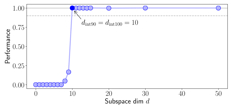
Plot of performance vs. subspace dimension for the toy example 2. The problem becomes both 90% solvable and 100% solvable at random subspace dimension 10, so $d{int90}$ and $d_{int100}$ are 10._
$d_{int}$ Details
- $d_{int100}$: solutions whose performance is statistically indistinguishable from baseline solutions
- $d_{int100}$ tends to to vary widely
- $d_{int100} \rightarrow D$ when the task requires matching a very well-tuned baseline model
- $d_{int90}$: solutions with performance at least 90% of the baseline
- More practical and useful
Experiments: MNIST
Compression
- FC and CNN are very compressible
- Store
- The random seed to generate the frozen $\theta^{(D)}$
- The random seed to generate $P$
- The 750 floating point numbers in $\theta^{(d)}_*$
- FC
- 750 degrees of freedom (0.4% params) for 90% of the baseline performance
- Assuming fp32, compression factor = 260x (from 793kB to only 3.2kB)
- CNN (LeNet)
- 290 degrees of freedom (0.65% params) for 90% of the baseline performance
- Assuming fp32, compression factor = 150x
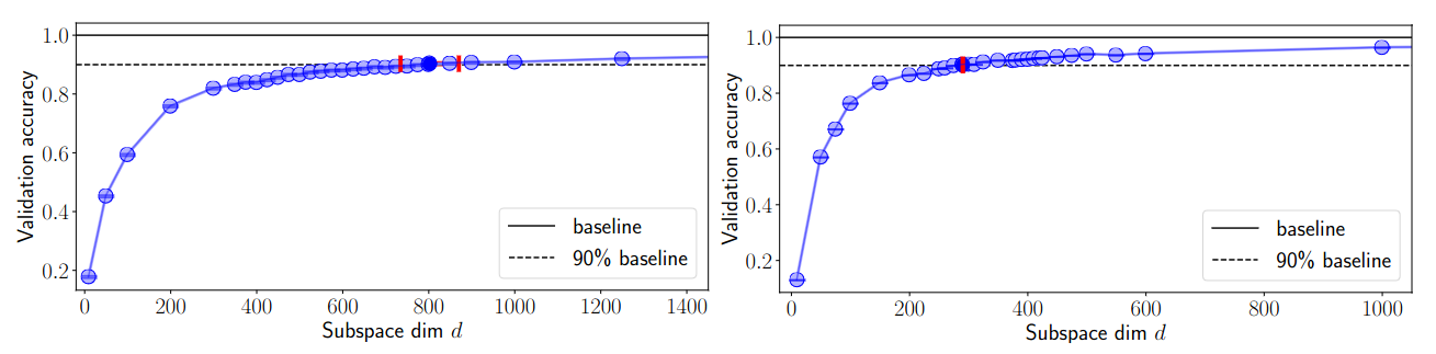
Performance (validation accuracy) vs. subspace dimension d for two networks trained on MNIST. Left: FC; Right: CNN.
Robustness of Intrinsic Dimension
- How intrinsic dimension varies across FC networks with a varying number of layers and varying layer width
- Grid sweep on FC
- Layers $L \in {1, 2, 3, 4, 5}$
- Width $W \in {50, 100, 200, 400}$
- Results
- $D$ changes by a factor of 24.1
- $d_{int90}$ changes by a factor of 1.33
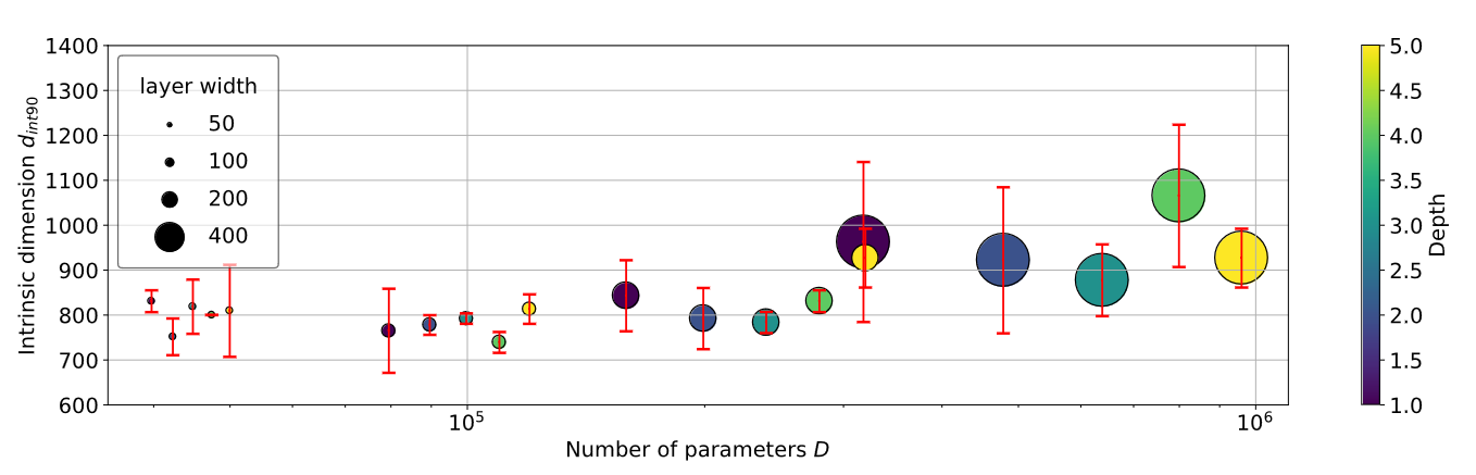
Intrinsic dimension vs number of parameters for 20 FC models. Though the number of native parameters $D$ varies by a factor of 24.1, \(d_{int90}\) varies by only 1.33. This indicate that \(d_{int90}\) is a fairly robust measure across a model family.
Random Subspaces Parameter Efficiency
- If the intrinsic dimension for MNIST is low, can we directly train a small network, instead of train in subspace of large network?
- 1000 small networks
- Layers $L \in {1, 2, 3, 4, 5}$
- Width $W \in {2, 3, 5, 8, 10, 15, 20, 25}$
- Results
- FC: Given the same level of validation accuracy, there persistent horizontal gap given similar # of trainable parameters
- CNN: generally more parameter efficient than FC
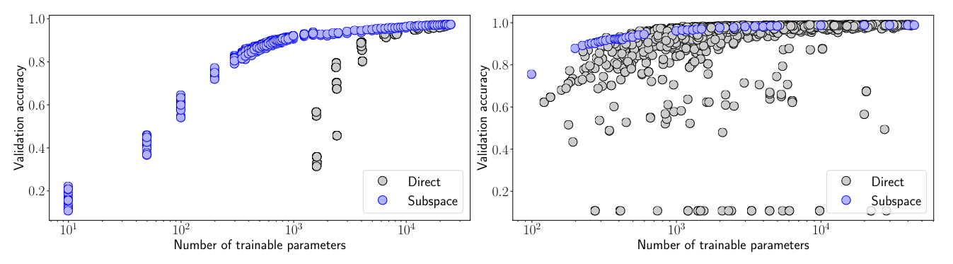
Performance vs. number of trainable parameters for (left) FC networks and (right) CNN trained on MNIST. Gray circles: randomly generated direct networks. Blue circle: random subspace training results. CNN: parameter efficiency varies, as the gray points can be significantly to the right of or close to the blue manifold.
Measuring $d_{int90}$ on Shuffled Data
- Compared to FC, CNN impose inductive bias. So are CNN always better than FC on MNIST?
- Shuffled Data: pixels are subject to a random permutation, chosen once for the entire dataset
- Results
- FC: $d_{int90}$ remains at 750
- CNN: $d_{int90}$ jump from 290 to 1400
- Catch
- CNN better suited to classifying digits given images with local structure
- When this structure is removed, violating convolutional assumptions, more degrees of freedom are now required to model the underlying distribution
Experiments: Various Learning Problems
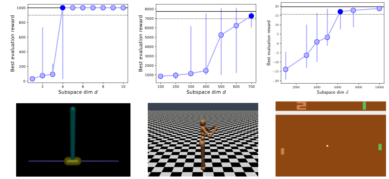
Intrinsic dimensions on InvertedPendulum−v1, Humanoid−v1, and Pong−v0. This places the walking humanoid task on a similar level of difficulty as modeling MNIST with a FC network. Pong on the same order of modeling CIFAR-10.
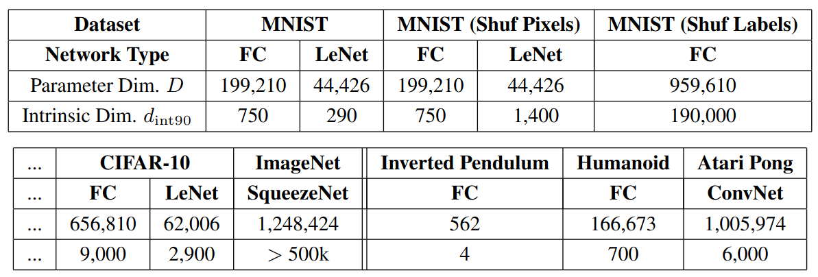
\(d_{int90}\) measured on various supervised and reinforcement learning problems.