Quantization: 8-bit
This post is mainly based on
- A Survey of Quantization Methods for Efficient Neural Network Inference, 2021
- LLM.int8(): 8-bit Matrix Multiplication for Transformers at Scale, 2022
- LLM.int8() implementation: bitsandbytes
- Designed for training
- Not efficient / low GPU utilization in inference
- High-performance implementation: EETQ
- GEMM kernels for optimized matrix multiplication
- Flash-Attention for optimized attention layer
Overview & Survey
- Quantization: map from input values in a large (often continuous) set to output values in a small (often finite) set, e.g., FP32 -> INT8
- Error measure
- Forward error: $\Delta y = y^* − y$
- Backward error: the smallest $\Delta x$, s.t., $f(x + \Delta x ) = y^*$
- Advantage: reduce the memory footprint and improve speed
- Why Quantization is Hard? Answer: Certain algorithms that solve that problem “exactly” in some idealized sense perform very poorly in the presence of “noise” introduced by the peculiarities of roundoff and truncation errors
A Concrete Example
Quantization in Neural Nets
- Different needs: training vs inference
- Classical quantization research: compression (find a 2-way mapping between original model and compressed model)
- Most current neural net models are heavily over-parameterized
- NNs are very robust to aggressive quantization
- People care about forward error (e.g., predict label / accuracy)
- Possible to have high error/distance between a quantized vs original model, while still attaining very good generalization performance
- Problem setup
- Given trained model parameters $\theta$ in FP32
- Reduce the precision of both
- The model parameters $\theta$
- The intermediate activation maps $h_i, a_i$
- Goal: minimal impact on the generalization power/accuracy of the model
Uniform Quantization
\[Q(r) = \operatorname{Int}(r/S) - Z\]where:
- $Q$: the quantization operator
- $r$: a real valued input (activation or weight)
- $S$: a real valued scaling factor
- $Z$: an integer zero point
More on Scaling Factor $S$:
\[S = \frac{\beta - \alpha}{2^b-1}\]- Determined by clipping range $[\alpha, \beta]$ and bit-width $b$
- For symmetric quantization, $Z = 0$
Quantization Variants
- Dynamic Quantization: Computes the clipping range of each activation and store a map
- Quantization Granularity: Layerwise Quantization / Channelwise Quantization
- Quantization-Aware Training: quantization is performed in training
- Post-Training Quantization: quantization is performed after training, may require a small set of training data to improve quantization quality
Quantization-Aware Training (QAT)
- What is QAT?
- Forward and backward pass are performed in FP
- Model parameters are quantized to INT after each gradient update
- Performing the backward pass with floating point is important, as accumulating the gradients in quantized precision can result in high error
- Non-Differentiable Operator
- Quantization operator is a piece-wise flat operator
- Non-differentiable!
- Straight Through Estimator (STE)
- Approximate the gradient of Quantization operator with an identity function
- Often works well in practice, except for ultra low-precision quantization (binary quantization)
- This re-training may need to be performed for several hundred epochs to recover accuracy
Post-Training Quantization (PTQ)
- What is PTQ?
- Adjust NN parameters without re-training
- Advantage of PTQ
- Low compute overhead
- Can be applied when data is limited or unlabeled
- Lower accuracy compared to QAT
- Mitigation
- Bias correction
- Equalizing the weight ranges
- Analytically computes the optimal clipping range and the channel-wise bitwidth
- Optimizing the L2 distance between the quantized tensor and the corresponding floating point tensor
- Some techniques may need access to training data
LLM.int8(): 8-bit Matrix Multiplication for Transformers at Scale
- A two-part quantization procedure
- Step 1: Vector-wise Quantization
- Matrix multiplication can be decompose into inner products of row and column vectors
- For each row / column, define a quantization normalization constant (to retain higher precision)
- Then denormalize to recover the true scales
- Step 2: Mixed-precision Decomposition Scheme
- Goal: handle outliers in hidden layers
- For outlier dimensions: perform 16-bit matrix multiplication (0.1% of values)
- For Non-outlier dimensions: perform 8-bit matrix multiplication (99.9% of values)
Challenge of Quantization for LLM
- Need for higher quantization precision at scales beyond 1B parameters
- Each inner products of row and column vectors may have different scale
- Need to explicitly represent the sparse but systematic large magnitude outlier features
- These outliers emerge in all transformer layers starting at scales of 6.7B parameters
- These outliers ruin quantization precision
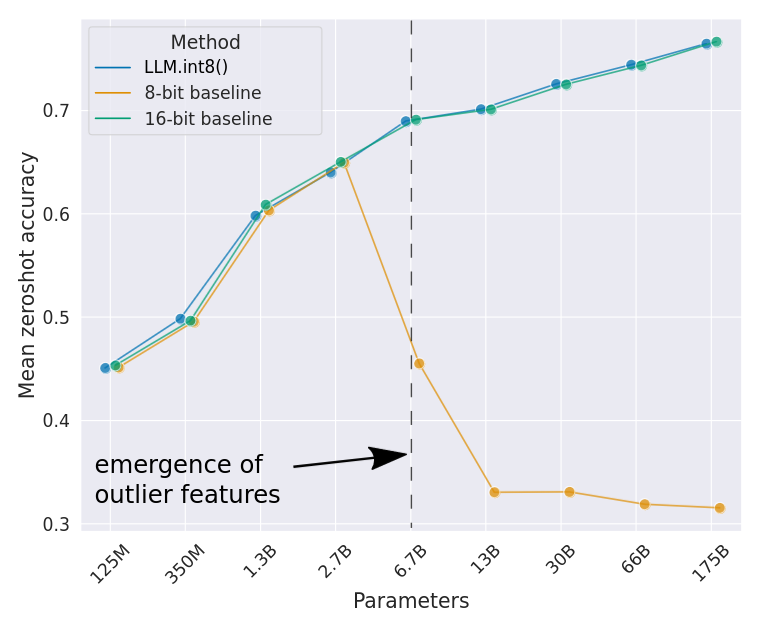
OPT model mean zeroshot accuracy decreases for quantized model beyond 6.7B parameters. This coincide with systematic outliers occurrence in model beyond of 6.7B parameters.
Outliers
- As we scale transformers to 6B parameters
- Large features with magnitudes up to 20x larger than in other dimensions first appear in about 25% of all transformer layers
- Then gradually spread to other layers
- At around 6.7B parameters
- A phase shift occurs
- All transformer layers and 75% of all sequence dimensions are affected by extreme magnitude features
- Highly systematic occurrence
- At the 6.7B scale, ~150,000 outliers occur per sequence
- Concentrated in only 6 feature dimensions across the entire transformer
- Importance of retaining outliers
- Setting these outlier feature dimensions to zero
- Decreases top-1 attention softmax probability mass by more than 20%
- Degrades validation perplexity by 600-1000%
- Despite them only making up about 0.1% of all input features
- Setting the same amount of random features to zero
- Decreases the probability by a maximum of 0.3% and degrades perplexity by about 0.1%
- Setting these outlier feature dimensions to zero
LLM.int8() Quantization
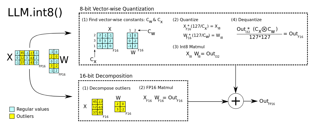
Given 16-bit floating-point inputs and weights, the features and weights are decomposed into sub-matrices of large magnitude features and other values. The outlier feature matrices are multiplied in 16-bit. All other values are multiplied in 8-bit, with vector-wise scaling.
Vector-wise Quantization
- Overview
- For each matrix product of hidden state $X_{f16}$ and weight $W_{f16}$
- Goal: find custom scaling constant for $c_x$ and $c_w$ for each row of $X_{f16}$ and columns of $W_{f16}$
- Decompose Matrix Multiplication
- Matrix multiplication = inner products of row and column vectors
- Therefore, we can use a separate quantization normalization constant for each inner product to improve quantization precision
- To recover the scales, we can de-normalize by the outer product of column and row normalization constants before we perform the next operation
- With just Vector-wise Quantization, it is possible to retain performance at scales up to 2.7B parameters
Mixed-Precision Decomposition
- Overview
- To handle the extreme outliers in the feature dimensions of the hidden states
- Deliver on high precision multiplication for these particular dimensions
- Mixed-Precision Decomposition
- Given hidden state $X_{f16} \in \mathbb{R}^{s \times h}$
- Outliers occur in all $s$ but in specific $h$
- Define a set for outlier feature dimensions $ O = \{ i | i \in \mathbb{Z}, 0 \leq i \leq h \} $
- $O$ contains all dimensions of $h$ which have at least one outlier with a magnitude larger than the threshold $\alpha$
- Matmul for $h \in O$ in performed in fp16; Matmul for $h \not\in O$ in performed in int8
- Findings
- $\alpha = 6.0$ is sufficient to reduce transformer performance degradation close to zero
Where $S_{f16}$ is the de-normalization term
Main Results
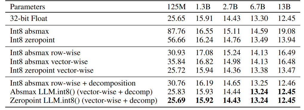
C4 validation perplexities of quantization. LLM.int8() is competitive wth full precision perplexities.
Outlier Features
- Observation
- Up to 150k outliers exist per 2048 token sequence for a 13B model
- Outlier features only represent at most 7 unique feature dimensions $h_i$
- Define outliers
- The magnitude of the feature is at least 6.0
- Affects at least 25% of layers
- Affects at least 6% of the sequence dimensions
Measuring the Effect of Outlier Features
- LMF = large magnitude features
- Emergence of LMF across all layers occurs suddenly between 6B and 6.7B parameters
- Percentage of layers affected increases from 65% to 100%
- Number of sequence dimensions affected increases rapidly from 35% to 75%
- This sudden shift co-occurs with the point where quantization begins to fail
- Emergence of LMF across all layers fits an exponential function of decreasing perplexity
- Indicate: Emergence of LMF is not only about model size but about perplexity
- Perplexity is related to additional factors (training data size, data quality)
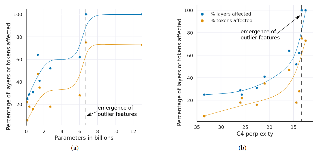
% of layers and all sequence dimensions affected by large magnitude outlier features across the transformer by (a) model size or (b) C4 perplexity.
More on Effect of Outlier Features
- Median outlier rapidly increases once outlier features occur in all layers
- The outliers and their asymmetric distribution disrupts Int8 quantization precision
- Core reason why quantization methods fail starting at the 6.7B scale
- The range of the quantization distribution is too large
- Most quantization bins are empty
- Small quantization values are quantized to zero
- Hypothesize
- Regular 16-bit floating point training becomes unstable due to outliers beyond the 6.7B scale
- Easy to exceed the maximum 16-bit value 65535 by chance if you multiply by vectors filled with values of magnitude 60
- The number of outliers features increases with respect to decreasing C4 perplexity
- Indicate: model perplexity rather than mere model size determines the phase shift
- Hypothesize: model size is only one important covariate among many that are required to reach emergence
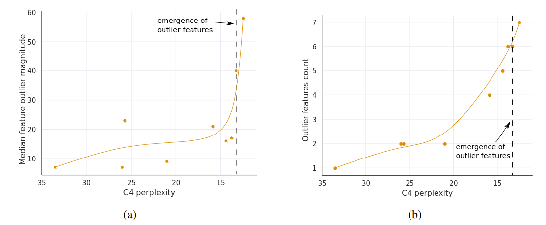
(a) Median magnitude of the largest outlier feature. (b) Number of outliers is strictly monotonic with respect to perplexity across all models analyzed.