LLM Scaling Law
This post is mainly based on
- Scaling Laws for Neural Language Models, OpenAI 2020
- Training compute-optimal large language model, DeepMind 2022
The goal is to present the methodology and considerations behind the scaling law, s.t. we can argue that LLM training is more of a science than art. We do not dig into details of each paper since:
- They are very long, and reader may only interested in specific part of the paper
- Their results could depend on dataset and dataset quality (signal-to-noise ratio)
- Selection of training hyperparameter depends on use case
- Training: all computing power is spent on training
- Inference: most computing power is spent on inference, which favors a smaller model
- They might be proved wrong or limited in future
Scaling Laws for Neural Language Models
- Loss scales as a power-law with
- Model size
- Dataset size
- Amount of compute used for training
- Network width or depth have minimal effects on loss
- The scaling law allow us to determine the optimal allocation of a fixed compute budget
- Larger models are significantly more sample efficient: optimally compute-efficient training involves training very large models on a relatively modest amount of data and stopping significantly before convergence
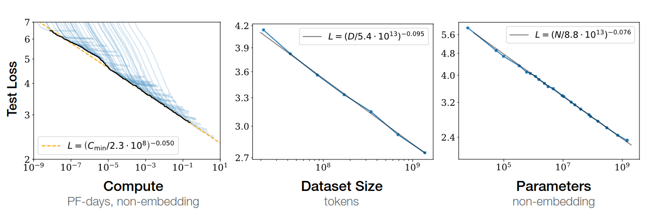
Empirical performance follows a power-law relationship with each individual factor when not bottlenecked by the other two.
Key Findings
- Testing loss can be modelled as a function
- Performance depends strongly on scale, weakly on model shape
- Testing loss follows smooth power law on scale
- Universality of overfitting
- Performance improves predictably as long as we scale up $N$ and $D$ together
- If we don’t scale up $N, D$, increasing other factors result in diminishing returns
- As we increase the model size $N$ 8x, we only need to increase the data $D$ by roughly 5x
- Transfer improves with test performance
- Validation loss is indicative of transfer learning performance
- Large models are more sample-efficient than small models
- Requires less compute and less data
- Training until convergence is inefficient
- When Compute budget $C$ is fixed, we attain optimal performance by training very large models and stopping significantly short of convergence
- Optimal scaling rate is $C^{0.74}/D$: data requirements $D$ growing very slowly vs compute $C$
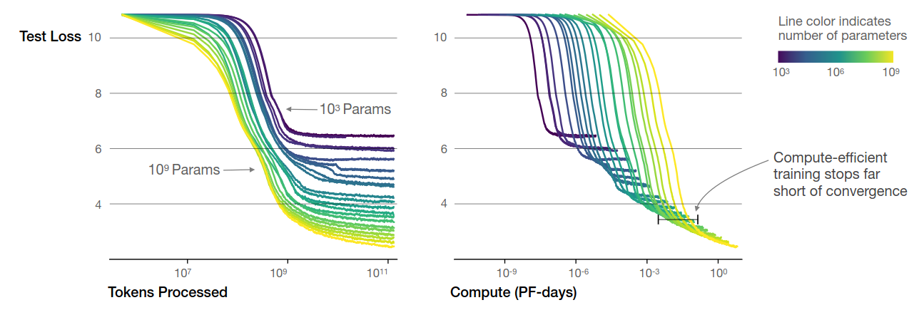
Left: Larger models require fewer samples to reach the same performance; Right: The optimal model size grows smoothly with the loss target and compute budget.
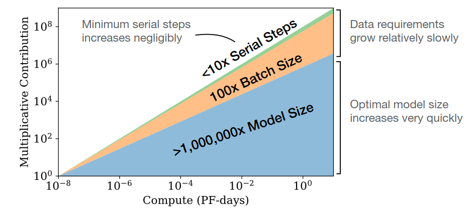
As we train with more compute, most of them are absorbed by larger model size and larger batch size. The serial step / training time increasing is not significant.
Notations (Section 1.3)
- $L$: cross-entropy testing loss
- $N$: number of model parameters (excluding all vocabulary and positional embeddings)
- $D$: size of the dataset (in tokens)
- $C = 6NBS$: amount of compute (in PF-days)
- $B$: batch size
- $S$: number of training steps
- $C = 10^15 \times 24 \times 3600 = 8.64 \times 10^19$ floating point operations
- $B_{crit}$: critical batch size for optimal tradeoff between time and compute efficiency
- $C_{min}$: estimated minimum amount of non-embedding compute to reach a given value of the loss
- To achieve $C_{min}$, we need batch size much less than the $B_{crit}$
- $S_{min}$: estimated minimum number of training steps to reach a given value of the loss
- To achieve $S_{min}$, we need batch size much greater than the $B_{crit}$
- $\alpha_X$: power-law exponents for the scaling of the loss as $L(X) \propto 1/X^{\alpha_X}$
- $N_C, D_C, C_C^{min}$ are constance with value defined om Scaling Laws below
Scaling Laws (Section 1.2)
Scaling Law 1. $L(N)$, given sufficiently large $D$ and $C$
\[L(N) = (\frac{N_C}{N})^{\alpha_N}\]where $\alpha_N = 0.076$ and $N_C = 8.8 \times 10^{13}$ non-embedding parameters
Scaling Law 2. $L(D)$, given sufficiently large $N$, early stopping
\[L(D) = (\frac{D_C}{D})^{\alpha_D}\]where $\alpha_D = 0.095$ and $N_C = 5.4 \times 10^{13}$ tokens
Scaling Law 3. $L(C_{min})$, given sufficiently large $D$, optimal size $N$ and sufficiently small batch
\[L(C_{min}) = (\frac{C_C^{min}}{C_{min}})^{\alpha_C^{min}}\]where $\alpha_C^{min} = 0.050$ and $C_C^{min} = 3.1 \times 10^{8}$ FP-days
The above relationship hold across
- 8 orders of magnitude in $C_{min}$
- 6 orders of magnitude in $N$
- 2 orders of magnitude in $D$
Coefficient $\alpha_X$ predicts the LLM performance improvement when we scale up $X$, e.g., when we double the number of parameters $N$, we can expect testing loss to reduce by $2^{-\alpha_N} = 0.95$.
$N_C, D_C, C_C^{min}$ depend on the vocabulary size and tokenization.
Batch Size Law. The critical batch size determines the speed/efficiency tradeoff for data parallelism, follows:
\[B_{crit}(L) = \frac{B_*}{ L^{1/\alpha_B} }\]where $\alpha_B = 0.21$ and $B_* = 2 \times 10^{8}$ tokens
How to use the Scaling Laws
Combining Scaling Law 1 and 2 we have:
\[D \propto N^{ \alpha_N / \alpha_D } \approx N^{0.74}\]i.e., as we increase the model size $N$ 8x, we only need to increase the data $D$ by roughly 5x
Experiments
- Training details
- Training dataset: WebText2 (65.86 GB uncompressed text)
- Vocab size: 50257
- Context length: 1024
- Models: Decoder only Transformer, LSTM, Universal Transformer
- Estimation of $N$
- $ N = 2 d_{model} n_{layer} (2d_{attn}+d_{ff}) = 12n_{layer}d_{model}^2 $
- Assuming $d_{attn} = d_{ff}/4 = d_{model}$
- Estimation of FLOPS
- See paper Table 1
- Generalization depends almost exclusively on the in-distribution validation loss
- See paper Figure 8
- Determine optimal dataset size
- See paper Equation 1.5-1.8 and Section 4.2
- To avoid overfitting when training to within that threshold of convergence we require $D \geq (5 \times 10^3)N^{0.74}$ many tokens
- Models smaller than $10^9$ parameters can be trained with minimal overfitting on the 22B token WebText2 dataset
- Dataset size may grow sub-linearly in model size while avoiding overfitting
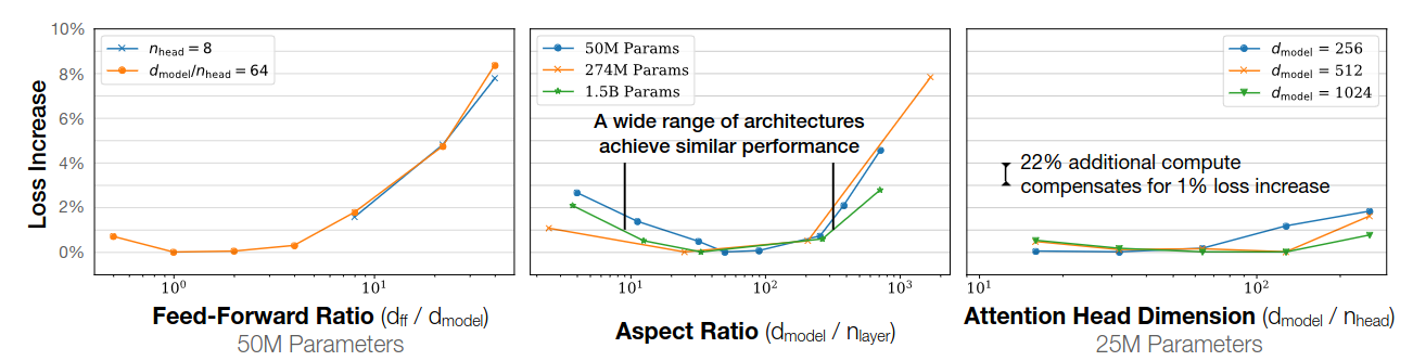 Performance depends weakly on model shape.
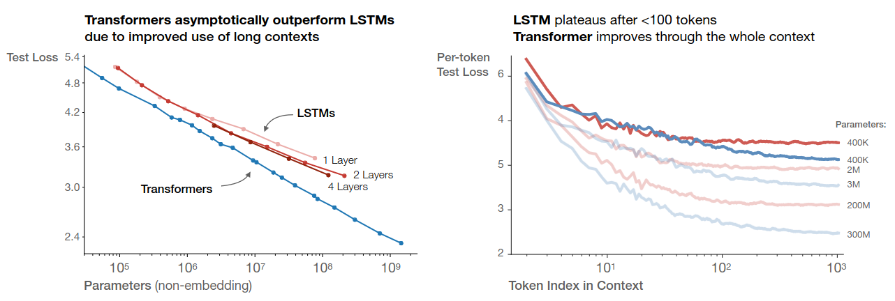 LSTM follows similar scaling law. However, transformer is more parameter efficient and exhibit no performance saturation on longer context.
Training compute-optimal large language model
- Recent LLMs are significantly under-trained
- Key findings: model size and the number of training tokens should be scaled equally
- Result
- Training of an model predicted by the new scaling law: Chinchilla-70B
- Chinchilla use same compute budget as Gopher, but trained on 4x more more data and 4x smaller in size
- Chinchilla uniformly and significantly outperforms Gopher-280B
- Chinchilla uses substantially less compute for fine-tuning and inference
In practice, the allocated training compute budget is often known in advance: how many accelerators are available and for how long we want to use them. Therefore, it is crucial to accurately estimate the best model hyperparameters for a given compute budget.
This paper present counter evidence to the Kaplan’s 2020 Scaling Law paper. The 2020 paper argues that there in a power law relationship: given a 10x increase computational budget, the size of the model should increase 5.5x while the number of training tokens should only increase 1.8x. This paper, however, find that model size and the number of training tokens should be scaled in equal proportions. This implies that most of the recently trained LLMs are significantly under-trained.
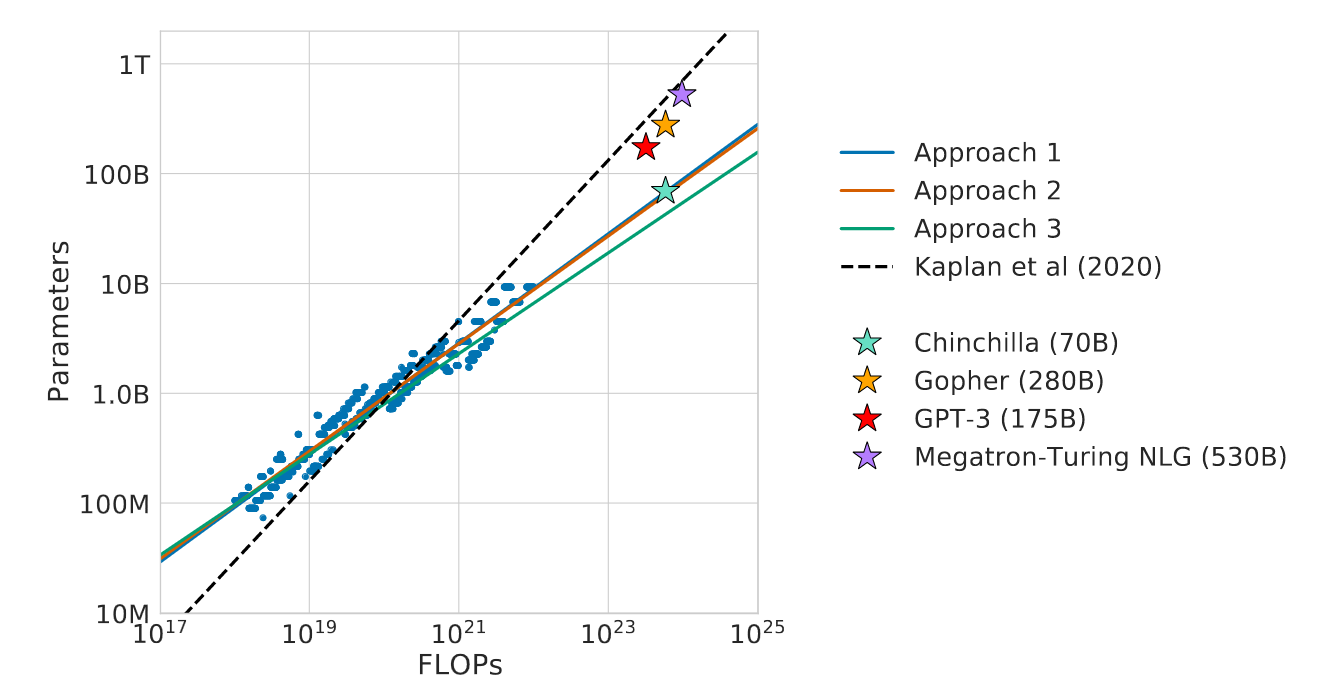
We overlay the predictions from our three different approaches, along with projections from Kaplan et al. (2020). We find that all three methods predict that current large models should be substantially smaller and therefore trained much longer than is currently done.
Problem
Let $L(N,D)$ be the pre-training loss given model parameters $N$ and number of training tokens $D$. Since the amount of computation is determined by $N, D$, we write $FLOPs(N,D)$, which is capped by our compute budget. Then we have our optimization problem:
\[N^*(C), D^*(C) = \text{argmin}_{N,D, s.t., FLOPs(N,D) = C} L(N,D)\]$L$ is obtained by empirical estimation on 400 models, ranging from under 70M to over 16B parameters, and trained on 5B to over 400B tokens.
Estimating the Scaling Behavior
- Use 3 different methods to fit empirical estimator on training curves
- Assuming a power-law relationship
Approach 1: Fix model size and vary number of training tokens
- Model size range: 70M - 10B
- Each model is trained with 4 different training sequences
- Decaying learning rate by 10x over a horizon
- Horizon range by a factor of 16x
- From those runs, we can directly observe the minimum loss achieved for a given FLOPs
- FLOP-loss frontier (Left figure below)
- From the above FLOPs-loss scatter plot, we can determine which run/configuration achieves the lowest loss
- This construct a mapping: from any FLOPs $C$ to the most optimal choice of model size $N$ and number of training tokens $D$
- We did this for 1500 log spaced FLOPs values
- Estimate power coefficient
- $N^* \propto C^a$ (Middle figure below)
- $D^* \propto C^b$ (Right figure below)
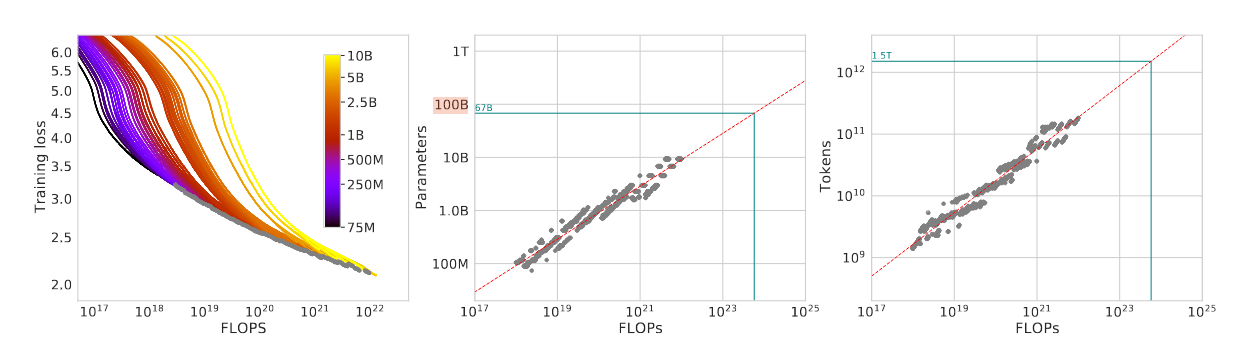
Left: FLOPS-loss frontier for all runs are is marked by grey points. Middle: log-scaled scatter plot for FLOPs vs model size $N$. Right: log-scaled scatter plot for FLOPs vs Training tokens $D$.
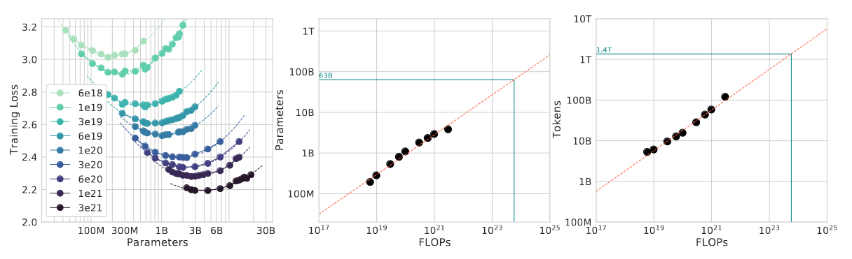
Approach 2: IsoFLOP profiles
- Fixed 9 different training FLOPs, vary model size
- FLOP counts range: $6 \times 10^{18} to 3 \times 10^{21}$
- This setup directly answered question “For a given FLOP budget, what is the optimal parameter count?”
- Estimate power coefficient
- Only 9 points available for estimation of power coefficient $a$ and $b$
- Some curvature in scatter plot indicate that power law may not be fully accurate
Approach 3: Fitting a parametric loss function
- Using all data from Approach 1 & 2
- Fit the parametric function below
where
- $E$: randomness in ground truth generative process / entropy of natural text
- $\frac{A}{N^\alpha}$: additional loss caused by a biased model (smaller model implies higher bias)
- $\frac{B}{D^\beta}$: additional loss caused by under-training / not train to convergence
For model fitting and mapping the parametric $\alpha$ and $\beta$ to $a$ and $b$, please read Section 3.3 of the paper.
Estimated Coefficients
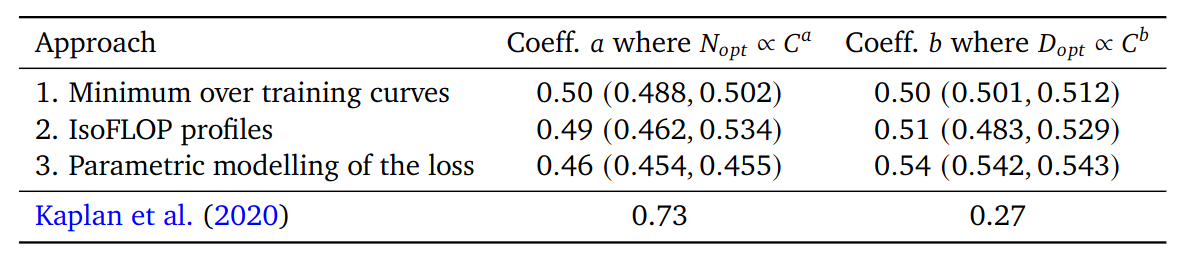
Our estimation of scaling law power coefficient vs Kaplan’s estimation.
Experiments
- Pile Evaluation: Chinchilla achieves a perplexity of 7.16 compared to 7.75 for Gopher
- MMLU: Chinchilla outperforms Gopher by 7.6% on average; performing better on 51/57 individual tasks, the same on 2/57, and worse on only 4/57 tasks.
- Reading comprehension: see table below
- BIG-bench: Chinchilla out performs Gopher on all but 4 BIG-bench tasks considered.
- TruthfulQA 0-shot: Chinchilla out performs Gopher by 43.6% to 29.5%
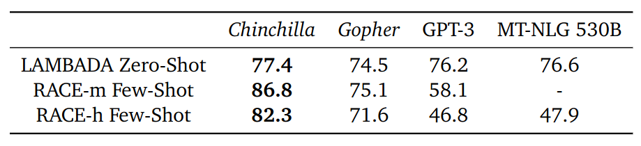
Reading comprehension performance of different LLMs.