Word Embedding
This post is mainly based on
- Efficient Estimation of Word Representations in Vector Space, ICLR 2013
- Distributed Representations of Words and Phrases and their Compositionality, NIPS 2013
- Linguistic Regularities in Continuous Space Word Representations
- word2vec Parameter Learning Explained
- Lilian Weng’s blog on word embedding
Prior to 2013, there were a lot of progress on mapping documents to vectors, using techniques like Latent Semantic Analysis (based on SVD) and Latent Dirichlet Allocation (based on non-negative matrix factorization and variational inference). One can image modifying the above method for word embeddings: replace the word-document matrix by word cooccruance matrix. However, LSA only captures principal components and LDA could be slow on large matrix. Little progress was made on finding scalable word embeddings.
Word2Vec was proposed in 2013 in a series of papers by Tomas Mikolov (It is interesting that Word2Vec is the just the name of the neural model they released in google code archive; none of the paper explicitly named their neural skip-gram architecture as Word2Vec). Although a bit falling out of fashion today, Word2Vec was a considered a break through in 2013, especially consider it enabled some simple algebra on the embedding space (although this kind of algebra is criticized, details here). The Negative Sampling technique it proposed also has profound impact and find applications in new fields like Contrastive Learning. Following Word2Vec, GloVe was proposed by Stanford NLP Group in 2014. GloVe is less scalable compared to Word2Vec, since it was based on matrix factorization.
Recent neural architecture is less reliant on pre-trained word embeddings, as deep learning framework like pytorch allows direct training of a word embedding though embedding layers. Embedding layer is essentially a look up table to a set of trainable parameters. Those trainable parameters are embeddings and can be optimized by automatic differentiation (this stackoverflow post has a good explanation).
Compared to Word2Vec, newer word embedding model like BERT and GPT generates contextual word embeddings: the output of individual word embedding changes according the context of the sentence.
We will only discuss Word2Vec in this post.
Word2Vec
I think the both the first and the second word2vec paper are not well written. If you are interested in details of word2vec, this paper: word2vec Parameter Learning Explained is a good resource. These two blogs offer an easier read:
Word2Vec maps a word to a vector or a representation. The author mentioned that their goal is to learn distributed representations of words. Geoffrey Hinton’s slides provides a definition for distributed representation in neural networks. I modified his definition for word embeddings:
- Each concept is represented by many dimensions in embedding space
- Each dimension in embedding space participates in the representation of many concepts
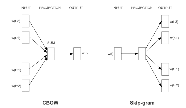
Two architectures are proposed: Continuous Bag-of-Words (CBOW) and Continuous Skip-gram (Skip-gram)
Assume we have a vocabulary size $V$, context word size $k$.
CBOW
- Task: predict the target word $w_t$ from $k$ context words $[ w_{c_1}, … w_{c_k} ]$
- $[ w_{c_1}, … w_{c_k} ]$ are mapped to their learnable embedding $[ \phi_{c_1}, …, \phi_{c_k} ]$, then averaged to $\bar{\phi}$
- Pass through a linear layer to get $[u_1, …, u_V]$
- Pass through a softmax layer to get distribution $P(w_1, … w_V | w_{c_1}, …, w_{c_k}) = [p_1, …, p_V]$
- Optimization goal: $\operatorname{argmax} \log P(w_t | w_{c_1}, …, w_{c_k}) $
Skip-gram
- Task: For $i = 1, …, k$ Predict the context word $w_{c_i}$ from the target word $w_t$
- The target word is mapped to its learnable embedding $\phi$
- Pass through a linear layer to get $[u_1, …, u_V]$
- Pass through a softmax layer to get distribution $P(w_1, … w_V | w_t) = [p_1, …, p_V]$
- Optimization goal: $\operatorname{argmax} \log P(w_{c_i} | w_t) $
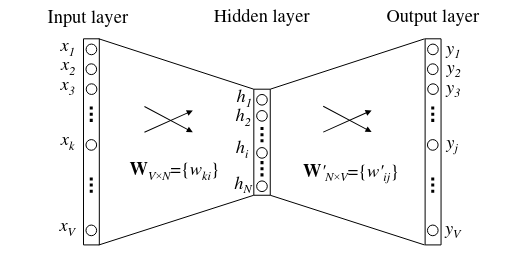
WLOG, consider above visualize the Skip-gram model. Some intuitions on the two linear layer:
- $W$ matrix
- Maps a one-hot encoded word to its embedding
- Row $i$ of $W$ correspond to the $i$-th word’s embedding
- $W’$ matrix
- Maps an embedding to unnormalized probability of context word
- $h^\top W’=$ vector of unnormalized probability of context word
- Row $j$ of $W’$ correspond to the $j$-th word’s probability
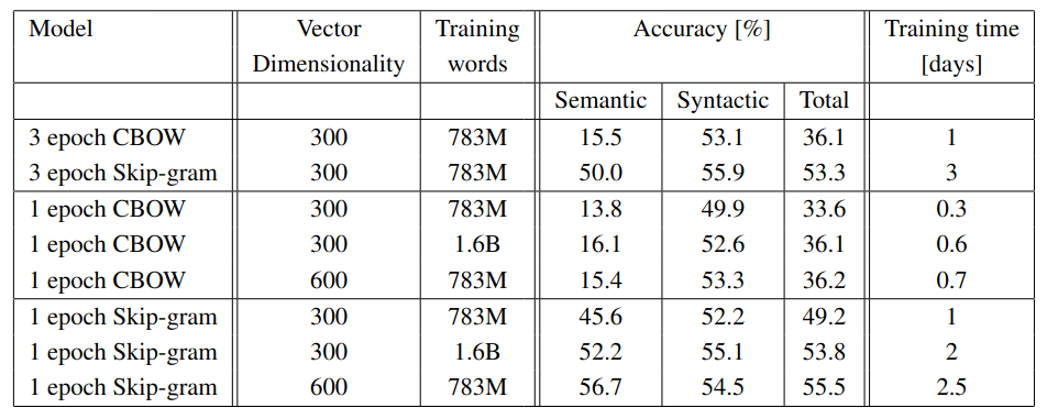
The result suggest that Skip-gram significantly outperforms CBOW in semantic tasks.
Optimization
WLOG, consider Skip-gram model: the optimization goal is maximizing the log likelihood $ \log P(w_{c_i} | w_t) $. Assuming $w_j$ is a context word of $w_t$, we can rewrite this optimization goal as minimizing the loss function $\mathcal{L}$, where $\mathcal{L}$ is defined as:
\[\begin{align} \mathcal{L} &= -\log P(w_{c_j} | w_t) \\ &= -\log p_j \\ &= -\log \frac{\exp(u_j)}{\sum \exp(u_i)} \\ &= -u_j + \log( \sum_{i=1}^V \exp(u_i) ) \end{align}\]Negative Sampling
Observed that the above optimization problem is computational expensive: the automatic differentiation needs to trace back the sum: $\log( \sum_{i=1}^V \exp(u_i) )$. For corpus with huge $V$, this is not efficient.
Observed the inefficient of the old loss function, we can propose a new loss function that sum over a small sample of $u_i$. This results in an equivalent optimization problem. The benefit is: instead of differentiate through all $u_i$, we can sample a few negative examples and differentiate through them. A formal explanation involves Noise Contrastive Estimation (NCE). You can refer to Lilian Weng’s blog for details.
An informal explanation is: to avoid $\log(\sum_{i=1}^V \exp(u_i))$, we need to change it to an expectation $\mathbb{E}[\log(u_i)]$ so that we can use sampling $w_i \sim P$ to solve the optimization problem. However, it is not clear how to take the sum to the outside of $\log$. Therefore, we take a bet and modified the optimization goal to:
\[\mathcal{L} = -\sigma(u_j) + \mathbb{E}_{w_i \sim P}[ \log \sigma(-u_i) ]\]where $\sigma$ is sigmoid function: $\sigma(x) = \frac{1}{1 + e^{−x}}$. This turns the $V$-class classification problem into a $2$-class classification problem $f(w_t, i) = 0 \text{ or } 1$ (if the $i$-th word is the context word of $w_t$). It also worked in practice. As previously mentioned, why this work involves the NCE argument.
The training data can be constructed as follow: for each target word $w_t$
- Positive Sample
- $k$ context words
- Ground truth label $f(w_t, i) = 1$
- Negative Sample
- $2k-5k$ words sampled from $P$
- Ground truth label $f(w_t, i) = 0$
The author find that empirically, setting the sampling distribution $P$ to the unigram distribution $U(w)$ raised to the 3/4rd power (i.e., $U(w)^{3/4}/Z$) yields the best performance.
Subsampling of Frequent Words
In very large corpora, the most frequent words can easily occur hundreds of millions of times (e.g., “in”, “the”, and “a”). Such words usually provide less information value than the rare words.
The authors modified the sampling probability $P(w_i)$ as follow:
\[P(w_i) = 1 - \sqrt{\frac{t}{f(w_i)}}\]where $f(w_i)$ is the frequency of word $w_i$ and $t$ is a chosen threshold (typically around $1e−5$).
Subsampling of frequent words results in a significant speedup (around 2x - 10x), and improves accuracy of the representations of less frequent words.
Distributed Representations in Semantic Space
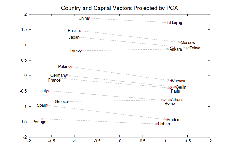
Two-dimensional PCA projection of the 1000-dimensional Skip-gram vectors of countries and their capital cities.