Transformer in Reinforcement Learning

This post is mainly based on

Background

Transformer has become the model of choice in for natural language processing (NLP) tasks and recently have also achieve state of art performance in computer vision (CV) tasks. However, its applications to reinforcement learning (RL) problems remain limited. In this article, we will review two recent attempts on applying transformers to solve RL problems.

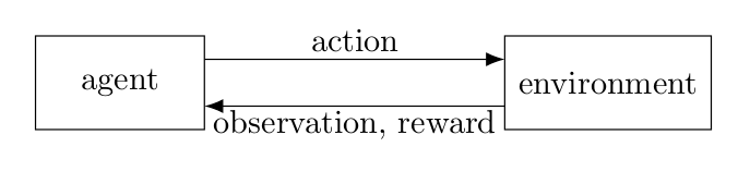
Recall that reinforcement learning aim to solve the sequential decision making problem. In the abstract form, the reinforcement learning involves an agent interacting with the environment. The agent observe current state $s_t$, sample an action $a_t$ and observe the reward $r_t$ and the next state $s_{t+1}$, where $t$ is the time step. The goal of the agent is to maximize the sum of (discounted) reward $R_t = \sum_{i=1}^t r_i$. We will refer to this setup as the standard form. Most of the existing RL research focus on the standard form, since there is theoretical guarantees on optimality based on Bellman equations (if you are interested in those theoretical guarantees, Akshay Krishnamurthy’s note is a good starting point).

Transformer

A standard NLP transformer receives the input as a set of token embeddings. It adds a positional encoding to the input embeddings and applys attention mechanism to retrieve a distributed representation of the input sequence. The attention mechanism select information that is “useful” for prediction tasks based on a set of learnable matrices: queries, keys and values.

RL Transformer

To apply transformer in a RL task, we first need to convert the RL environment into sequential data. Instead of viewing the sequential decision making problem in the standard form, we can “flatten” it into a trajectory, for example, $\tau = (s_0, a_0, r_0, s_1, a_1, r_1, …, s_T , a_T , r_T)$. Essentially, this convert the RL problem into a supervised learning problem (seq-to-seq prediction), therefore, we can train a transformer on $\tau$ to learn some target $(y_1, y_2, …, y_k)$. Two recent papers proposed their own version of “flatten” schema and this leads to two new RL algorithms: Decision Transformer and Trajectory Transformer.

Offline learning

To full utilize the parallelism of transformer, both paper limit the setting into offline learning: agent is given a set of trajectories, possibly from expert demonstrations or sub-optimal agents. Note that offline learning is challenging due to agent can only learn from trajectories in the training set without exploration: an agent can only learn the reward $r(s,a)$ from taking action $a$; it cannot choose action $a’$ to see the reward $r(s, a’)$. In testing environment, may not be able to replicate a trajectory or reach a previously observed state (e.g., stochastic environment $P(s,a)$ or different initial distribution $\mu$); this is called distribution shift. To learn an optimal policy, the agent need to generalize the experience it observed in training set. If you are not familiar with Offline Reinforcement Learning, Sergey Levine’s survey is a good starting point.

Decision Transformer

The author mentioned that one of the motivation of Decision Transformer (DT) is direct credit assignment: transformers can perform credit assignment directly via self-attention. In comparison, traditional TD-learning achieves credit assignment by Bellman backups, which “slowly propagate rewards and are prone to distractor signals.” The author also mention that transformer avoids the need for “discounting future rewards.”

Most of the theoretical results of RL relies on Markov assumption, which is unlikely to hold in practice. To create a proper representation of state space, feature engineering needs to be performed. For example, in Pong, at least 2 frames are required to compute the direction of the ball. Transformer is designed to handle sequential data and could possibly remove the requirement for Markov assumption or feature engineering.

Model

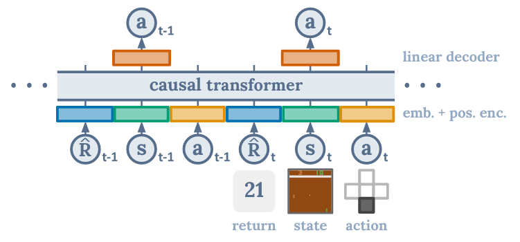
Trajectory representation: $\tau = (\hat{R}_1, s_1, a_1, \hat{R}_2, s_2, a_2, …, \hat{R}_T, s_T , a_T)$
Embedding:
- linear layer for each modality; learnable; projects raw inputs to the embedding dimension
- layer normalization
- For environments with visual inputs, the state is fed into a convolutional encoder instead of a linear layer
Positional encoding: learned embedding, one timestep corresponds to three tokens (for $(\hat{R}_i, s_i, a_i)$)
Model: GPT model
Prediction:
- Target: future action tokens $a_{t+1}$
- Loss: cross-entropy loss for discrete actions; MSE for continuous actions

Experiments

Environment

Atari tasks: Breakout, Qbert, Pong, and Seaquest
D4RL offline benchmark: gym’s HalfCheetah, Hopper, Walker, Reacher
Key-to-Door: trajectories generated by applying random actions (details)

Benchmark

TD learning
- CQL: Conservative Q-Learning
- BEAR: Stabilizing off-policy q-learning via bootstrapping error reduction
- BRAC: Behavior regularized offline reinforcement learning
- AWR: advantage-weighted regression: Simple and scalable off-policy reinforcement learning
Imitation learning
- BC: Behavior cloning

On 4 gym continuous control tasks, training was performed under different trajectory D4RL datasets. In “Medium” dataset, trajectories are generated by sub-optimal expert with 1/3 of score of an expert policy. In “Medium-Expert” dataset, half of the trajectories are generated by “Medium” and another half are expert demonstration.

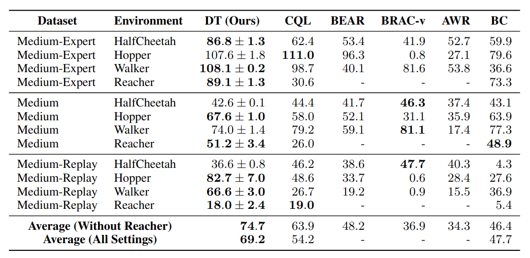
While Decision Transformer cannot dominate TD-based methods on all tasks, it still achieved the best average performance.

Ablation studies

Context window length

The context window length stands for the length of the input embedding into transformer. As previously mentioned, most Atria environment represented in single frame are likely non-stationary. The author compared the performance of DT under context window length K = 1 vs K = 30 (50 for Pong) and demonstrated that DT incorporating information previous K-1 states to achieve better performance.

Predicting future reward as an auxiliary task

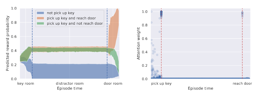
The author mentioned that they added predicting future states and rewards as auxiliary tasks in ablation studies. Although this does not improve the performance of agent (measuring by total rewards), it demonstrated that transformer can be used as a an effective critic (see Chapter 11 Actor–Critic Method of Sutton’s book) to perform credit assignment. In the Key-to-Door environment, the agent needs to take a key in room 1 without any reward and open a door in room 3 to accept an reward (It appears that they used a simplified Key-to-Door environment, and the agent does not receive any reward in the second room). The challenge for credit assignment is long-range dependency. The transformer learned to assign the credit to “pick up key” and “reach door” and you can see obvious changes in predicted reward probability.

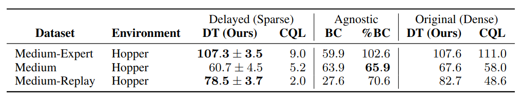
Dense vs sparse reward

Trajectories in D4RL benchmarks are reward dense, meaning that the agent receives densely populated rewards across the trajectory. However, this could be unrealistic and/or expensive in practice and may rely on reward engineering. TD method is known to suffer from the “hard exploration problem” and unable to propagate rewards to early states. One of the most promising result is sparse appears to have limited negative effect on Decision Transformer as shown in the table below.

Trajectory Transformer

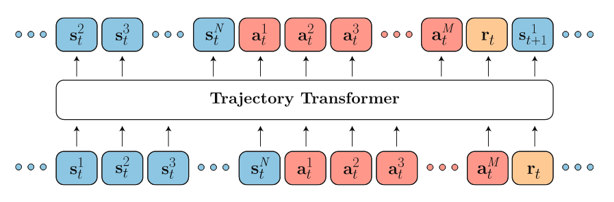
The Trajectory Transformer (TT) proposed a different “flatten” schema for trajectory $\tau$. Suppose $s_t$ is $N$-dimensional and $a_t$ is $M$-dimensional. Instead of obtaining embeddings for $s_t, a_t$, TT decompose the $s_t, a_t$ into their individual dimension $s_t^1, s_t^2, … s_t^N$ and $a_t^1, a_t^2, … a_t^M$. This turn the original length $T$ trajectory $\tau$ into length $T(N+M+1)$. Individual dimension (could be one of the $s_i^j, a_i^j$ or $r_i$) is then discretized into tokens (In fact, I don’t really understand why they want to convert $s,a,r$ into “same unit” and then learns an embedding on top of them. Please refer to the paper for details).

Model

Trajectory representation: $\tau = (…, s_t^1, s_t^2, … s_t^N, a_t^1, a_t^2, … a_t^M, …, r_t, …)$
Embedding: learnable a linear layer; projects size $V \times (N+M+2)$-dimensional token into 128-dimensional embedding
Positional encoding: Not discussed
Model: GPT model
Prediction
- Target: $V$-dimensional token (for $s, a, r$)
- Loss function: customized / log-likelihood
- \[\mathcal{L}(\tau)=\sum_{t=1}^{T}\left(\sum_{i=1}^{N} \log P_{\theta}\left(s_{t}^{i} \mid \mathbf{s}_{t}^{<i}, \boldsymbol{\tau}_{<t}\right)+\sum_{j=1}^{M} \log P_{\theta}\left(a_{t}^{j} \mid \mathbf{a}_{t}^{<j}, \mathbf{s}_{t}, \boldsymbol{\tau}_{<t}\right)+\log P_{\theta}\left(r_{t} \mid \mathbf{a}_{t}, \mathbf{s}_{t}, \boldsymbol{\tau}_{<t}\right)\right),\]
- where $\tau_{<t}$ to denote a trajectory from timesteps 0 through $t-1, s_{t}^{<i}$ to denote dimensions 0 through $i-1$ of the state at timestep $t$, and similarly for $a_{t}^{<j}$.

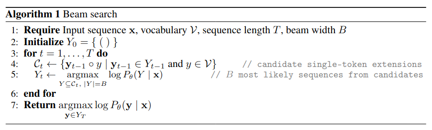
Planning The Trajectory Transformer takes an extra step to formalized the discussion on control, which was largely omitted by the Decision Transformer paper. They first described how to combine Beam Search and the Trajectory Transformer to solve control problem (see Algorithm 1). If you are not familiar with Beam Search, here is a good source.

Goal of control

Imitation learning
- Exactly Algorithm 1
Goal-conditioned reinforcement learning
- Change the optimization to $\operatorname{argmax} P_{\theta}\left(s_{t}^{i} \mid s_{t}^{<i}, \tau_{<t}\right)$
Offline reinforcement learning
- Change the Transformer’s optimization to $\operatorname{argmax} R_t$, where $R_t$ is reward-to-go given current trajectories

Experiments

Imitation learning on the dataset generated by a trained humanoid policy
Offline reinforcement learning: D4RL offline benchmark
Goal-conditioned reinforcement learning: AntMaze (v0)

Imitation learning

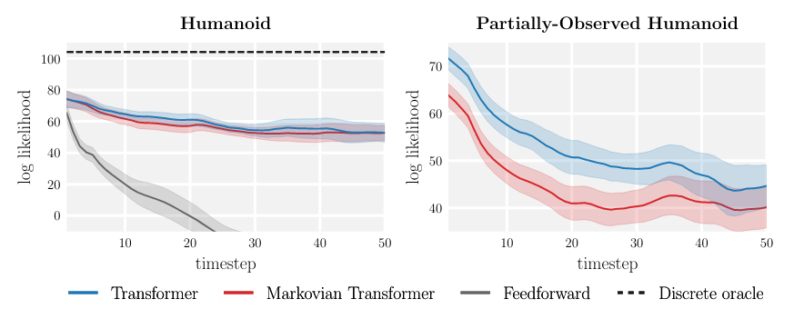
Below is a qualitative comparison of length-100 trajectories. Trajectories are generated Trajectory Transformer and state-of-the-art planning benchmark (denoted by Single-Step Model or Feed forward). Due to the compounding errors, the single-step model quickly accumulate prediction error which renders the agent unable to follow the expert demonstration after a few time steps.

Trajectory Transformer

Single-Step Model (feed forward Gaussian dynamics model from PETS)

Compounding model errors

In the partially-observed humanoid environment where every state is masked out with $50\%$ probability. the agent performed considerable worse, likely due to unable to retrieve all information from the past. This demonstrate the importance of considering long-horizon dependency and non-Markovian nature of the environment.

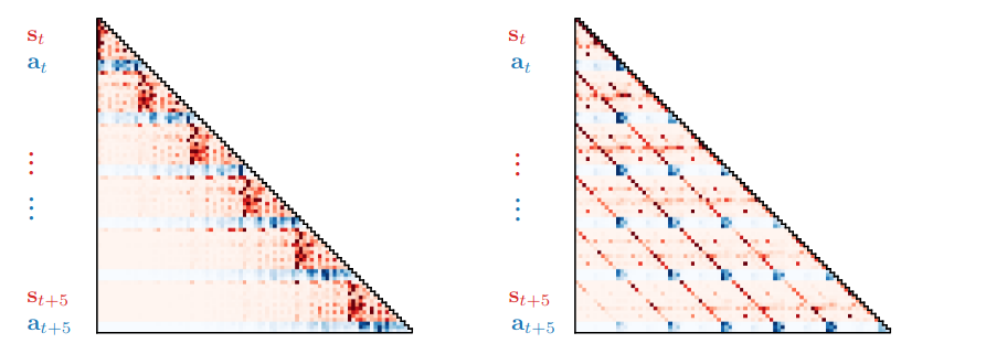
Attention patterns Visualization the attention patterns. This shown that: apart from the Markovian attention pattern (left), there is also a striated attention pattern (right) which focused on retrieving information from past states. More attention patterns are available at here.

Trajectory Transformer also reached or exceeded state-of-art algorithms on Offline reinforcement learning and Goal-conditioned reinforcement learning tasks. Please refer the paper for more details.

Discussion

The above two papers demonstrated that transformer are able to deliver or exceed state-of-art performance in various RL tasks. The Decision Transformer present that it is possible to use transformer to tackle the credit assignment problem and the delayed/sparse reward problem in RL. The Trajectory Transformer show the advantage of incorporating long-horizon dependency into RL.

The authors categorize their work as investigations of if RL can be reframed as a supervised learning problem and solved by transformers. While transformers delivers promising results, their disadvantages also need to be highlighted: prediction with Transformers is currently slower and more resource-intensive, requiring up to multiple seconds for action selection when the context window grows too large and precludes application of real-time control.

In the Trajectory Transformer paper, the authors discussed their vision: we aim to replace as much of the RL pipeline as possible with sequence modeling, so as to produce a simpler method whose effectiveness is determined by the representational capacity of the sequence model rather than algorithmic sophistication. In contrast, most of the state-of-art RL agents are very complex and requires distinct architecture to solve their domain problem. For example, “actor-critic algorithms require separate actors and critics, model-based algorithms require predictive dynamics models, and offline RL methods often require estimation of the behavior policy.” If researcher could unify different model architectures into a single high high-capacity sequence model, it is possible to develop a transferable benchmark model like ResNet for CV tasks or BERT for NLP tasks. If you have backgrounds in RL, I strongly recommend you to read the first two sections of Trajectory Transformer paper where the authors delivered a much detailed discussion on their motivations.