Optimizer
This post is mainly based on
- Sebastian Ruder’s blog
- Momentum & Nesterov: On the importance of initialization and momentum in deep learning, PMLR 2013
- AdaGrad: Adaptive Subgradient Methods for Online Learning and Stochastic Optimization, JMLR 2011
- RMSProp: Geoffrey Hinton’s slides of RMSProp
- Adam: A Method for Stochastic Optimization, ICLR 2015
- AdamW: Decoupled Weight Decay Regularization
Some notations of the original paper have been changed to keep consistency within this post.
SGD
Stochastic gradient descent (SGD) is a first order optimization algorithms. Let $J$ be the loss function and $\nabla_\theta J(\theta)$ be the gradient of $J$ w.r.t. $\theta$ evaluated on batch data $\{(x_i,y_i), …, (x_{i+b},y_{i+b})\}$ and $\eta$ be the learning rate. SGD update rule is given by,
\[\theta_{t+1} = \theta_t - \eta \nabla_\theta J(\theta_{t})\]Since gradient of SGD (stochastic gradient) is evaluated on batch data, we only have a noise estimation of the true gradient at each step.
\[\nabla_\theta J(\theta) = \mathbb{E}[ \nabla_\theta J(\theta; \{(x_i,y_i), ..., (x_{i+b},y_{i+b})\})]\]Therefore, it is unclear if we can converge a local minimum up to $\varepsilon$ accuracy with this stochastic gradient. Theoretical results on SGD convergence can be obtained by Robbins–Siegmund theorem, which is an analogy of Robbins-Monro algorithm. In short, if we set $\eta$ to decay at an appropriate rate, convergence can be achieved:
\[\sum_{i=1}^\infty \eta_i = \infty\] \[\sum_{i=1}^\infty \eta_i^2 < \infty\]More discussion can be found here
Vanilla SGD could be inefficient when $J(\theta)$ is not well shaped. For example, presence of local minimum/saddle points or oscillating path (gradient in one dimension is much larger than that in other dimensions). Variants of SGD have been proposed and some are widely used in practice.
Momentum & Nesterov
Momentum is a simple idea to tackle the above problem. Consider $\theta$ as location, $v_t$ as velocity, gradient $\nabla_\theta J$ as acceleration and $\gamma$ as friction. Given unit mass, relationship between velocity and acceleration are equivalent that of momentum and force. Then the update rule is,
\[v_{t+1} = \gamma v_t - \eta \nabla_\theta J( \theta_t)\] \[\theta_{t+1} = \theta_t + v_{t+1}\]SGD struggle to escape local minimum/saddle points, due to the gradient are close to zero. SGD with momentum can easily escape saddle points from velocity accumulated from previous gradient. For oscillating path, the gradients in y-axis will cancel each other while the gradients x-axis will accumulate into velocity, resulting in faster convergence.
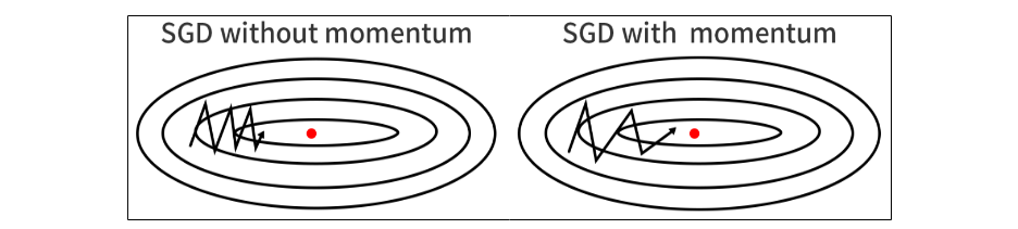
Image: momentum paper
Note than pytorch has a slightly different implementation of the update rule, where $\eta$ is applied to $v_t$ instead of $\nabla_\theta J( \theta_t)$:
\[v_{t+1} = \gamma v_t - \nabla_\theta J( \theta_t), \theta_{t+1} = \theta_t + \eta v_{t+1}\]Nesterov is similar to Momentum, except the gradient is evaluated at the next approximate location $\theta_t + \gamma v_t$. The idea is avoid overshooting: suppose the ball is rolled into the bottom of pit and the gradient is about to change the direction. SGD with Momentum will still accelerate at current update, but SGD with Nesterov will decelerate. On a general smooth convex functions $J$ with deterministic gradient, Nesterov achieves a global convergence rate of $O(\frac{1}{T^2})$ compared to $O(\frac{1}{T})$ rate for Gradient Descent
Additional readings:
- On the importance of initialization and momentum in deep learning
- The Frontier of SGD and Its Variants in Machine Learning
AdaGrad
The idea of AdaGrad is that each parameter $\theta_i$ should be assigned it own learning rate $\eta_i$. Consider the function $J(\theta) = \theta_1^2 + 100\theta_2^2$. The contour of $J$ is similar to the oscillating path plot in Momentum section. The problem of SGD is that learn rate $\eta$ does not match the geometry of the surface: starting from, say (10,10), the partial derivative $\frac{\partial J}{\partial \theta_2}$ is 100x bigger than $\frac{\partial J}{\partial \theta_1}$. Therefore, we would want learn rate $\eta_2$ be $\frac{1}{100}$ of $\eta_1$. However, the learn rate assign by vanilla SGD is the same for both parameters, resulting the oscillating path.
AdaGrad solve this problem by using accumulating gradient to estimate the geometry of $J$. The original idea involves using Subgradient Methods to obtain a better convergence rate. Define a adaptive adjustment matrix $G_t$ as a diagonal matrix where
\[G_{t, ii} = G_{t-1, ii} + (\frac{\partial}{\partial \theta_i} J(\theta_t))^2\]$G_t$ is the accumulation of past past gradient along $\theta_i$. The update rule is:
\[\theta_{t+1} = \theta_t - \frac{\eta}{\sqrt{G_t + \varepsilon}} \cdot \nabla_\theta J( \theta_t)\]where $\varepsilon$ improves the numerical stability of inverting the diagonal matrix, and $\eta$ is the base learning rate. $\frac{\eta}{\sqrt{G_t + \varepsilon}} \cdot \nabla_\theta J( \theta_t)$ is a matrix multiplication.
A simplified interpretation is: if $\theta_i$ frequently appears or $\theta_i$ is large, then dividing $\sqrt{G_t}$ will impose a lower adaptive learning rate; if $\theta_i$ is sparse or $\theta_i$ is small, then dividing $\sqrt{G_t}$ will impose a higher adaptive learning rate.
A well known problem of AdaGrad is that learning rate collapsed to zero: As learning progress and more gradient accumulated to $G_t$, $\frac{1}{\sqrt{G_t + \varepsilon}} \rightarrow 0$.
Additional readings:
RMSProp
RMSProp is modification of AdaGrad. The idea is: to avoid learning rate collapsed to zero, change the “accumulate gradient” strategy to “accumulate exponential decay of gradient”. Everything is the same as AdaGrad except calculation of $G_t$:
\[G_{t, ii} = \rho G_{t-1, ii} + (1-\rho)(\frac{\partial}{\partial \theta_i} J(\theta_t))^2\]More discussion can be found at Geoffrey Hinton’s slides.
Adam
The idea of ADAptive Moment estimation (Adam) is to apply to RMSProp’s adaptive learning rate on SGD with momentum. The authors mentioned that Adam’s magnitudes of parameter updates are invariant to rescaling of the gradient, and its stepsizes are approximately bounded by the stepsize hyperparameter. This possibly makes it less sensitive to choice of learning rate: in experiment, Adam performed equal or better than RMSProp, regardless of hyper-parameter setting.
We have change the Adam paper’s notations ($\alpha \rightarrow \eta$, $m_t \rightarrow v_t$, $v_t \rightarrow G_t$) maintain consistency in our post.
First, accumulate velocity on $v_t$ and accumulate squared gradient on $G_t$, with exponential moving averages. $\beta_1$ and $\beta_2$ are decaying factor for $v_t$ and $G_t$.
\[v_t = \beta_1 m_{t-1} + (1-\beta_1) \nabla_\theta J(\theta_{t-1})\] \[G_t = \beta_2 v_{t-1} + (1-\beta_2) [\nabla_\theta J(\theta_{t-1})]^2\]Seconds, perform initialization bias correction. The authors added this step due to $m_t$ and $v_t$ are biased toward zero at the first few updates, leading to small steps. $t$ is time step.
\[\hat{v}_t = \frac{v_t}{1-\beta_1^t}\] \[\hat{G}_t = \frac{G_t}{1-\beta_2^t}\]Third, update location $\theta$ with base learning rate $\eta$:
\[\theta_t = \theta_{t-1} - \frac{\eta}{\sqrt{\hat{G}_t} + \varepsilon} \hat{v}_t\]The author mentioned that good default hyperparameters are: $\alpha = 0.001, \beta_1 = 0.9, \beta_2 = 0.999, \varepsilon = 10^{−8}$
Reference: Adam: A Method for Stochastic Optimization
Comparison of optimizers
Optimization near a saddle point
SGD fails to make much progress. Adaptive learning rate methods and momentum based methods is able to escape from the saddle point.
Reference
Adaptive learning rate methods vs momentum based methods
Due to the large initial gradient, momentum based methods overshoot. Adaptive learning rate methods converge faster.
Reference
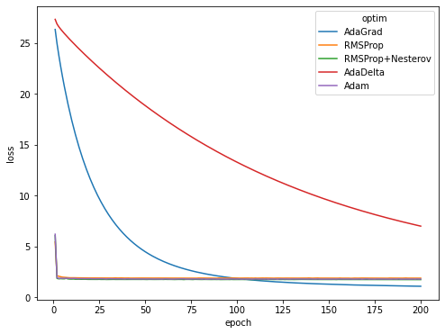
Converge on CV task
Rate of convergence of AdaGrad, RMSProp, RMSProp+Nesterov, AdaDelta, Adam on CIFAR-10 dataset. RMSProp and Adam significantly outperforms other methods on this task in convergence speed.
AdamW
[TBD]