CKConv: Continuous Kernel Convolution
This post is mainly based on
Conv vs CKConv
- Conv kernel
- Parameterized by a sequence of independent weights
- CKConv kernel
- Parameterized by a small neural network
- Modeled as a continuous function
- The continuous kernel is only discretized when you need to * it with discrete data sampled from continuous signal
CKConv and Attention Mechanism
In Attention Mechanism, given a sentense of length $n$: $(x_1, x_2, …, x_n)$, token $x_i$’s embedding $\phi(x_i)$ can be viewed as:
\[\phi(x_i) = \sum_{j=1}^n \alpha_j v_j\]Where the weights $\alpha_{i, j}$ associated with $v_j$ can be seen as dynamically generated parameters for each token $x_i$. The function that generate those $\alpha_{i, j}$ for $j = 1, …, n$ are parameterized by a neural network $\psi(x_i, x_{1:n})$.
In CKConv, parameters of convolution filter can be seen as dynamically generated for each timestamp $\Delta \tau_i$. The function that generate those $\psi(\Delta \tau_i)$ are parameterized by a neural network $\psi(t)$.
CKConv
- Convolutional Kernel = a small neural network
- CKConv Can define arbitrarily large memory horizons within a single operation
- Do not rely on any form of recurrence
- CKCNNs can be trained in parallel
- CKCNNs do not suffer from vanishing / exploding gradients or small effective memory horizons
- Can be evaluated at arbitrary positions
- CKConvs and CKCNNs can be used on irregularly sampled data
Background
Continuous Kernel
- Motivation: to handle irregularly sampled data
- Discrete convolutions
- Learn independent weights for specific relative positions
- Cannot effectively handle irregularly sampled data
Convolution Kernel Parameterization
Notation
- $[n]$: set ${0, 1, …, n}$
- $x, W$: vector and matrices
- $x_c$ sub-index of a vector
- $x(\tau)$: vector as function of time $\tau$
- $\mathcal{X}$: sequence ${x(0), x(1), …, x(N_X)}$
Centered and Causal Convolutions
Given continuous $x(t)$ and $\psi(t)$:
- $x: \mathbb{R} \to \mathbb{R}^{N_{\text{in}}}$, a vector valued signal on time
- $\psi: \mathbb{R} \to \mathbb{R}^{N_{\text{in}}}$, a vector valued kernel on time
The convolution is defined as:
\[(x * \psi)(t) = \sum_{c=1}^{N_{\text{in}}} \int_\mathbb{R} x_c(\tau) \psi_c(t-\tau) d\tau\]In practice, the signal $x$ is gathered as discrete input via some sampling procedure:
- $\mathcal{X}={x(\tau)}_{\tau=0}^{N_X}$
- $\mathcal{K}={\psi(\tau)}_{\tau=0}^{N_X}$
Centered Convolution:
\[(x * \psi)(t) = \sum_{c=1}^{N_{\text{in}}} \sum_{\tau=-N_{X/2}}^{N_{X/2}} x_c(\tau) \psi_c(t-\tau)\]Causal Convolution:
\[(x * \psi)(t) = \sum_{c=1}^{N_{\text{in}}} \sum_{\tau=0}^{t} x_c(\tau) \psi_c(t-\tau)\]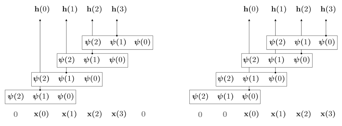
Visualization of. Left: centered Conv. Right: Causal Conv.
If $x(\tau)$ falls outside of $\mathcal{X}$, $x(\tau)$ is often padded by $0$.
Discrete Convolutional Kernels
Most convolutional kernels $\psi$ are parameterized $N_K + 1$ independent learnable weights.
$N_K$ must be kept small to keep the parameter count of the model managable. Hence, the kernel size is often much smaller than the input length: $N_K \ll N_X$.
This parameterization has many limitations:
- Kernel size $N_K$ must be defined a priori
- Implicitly assumes output only depends on past $\tau = N_K$ inputs
Dilated Convolutional Kernels
To increase receptive field and keep number of parameters in check, previous works propose to interleave kernel weights with zeros, to create dilated convolutional kernels.
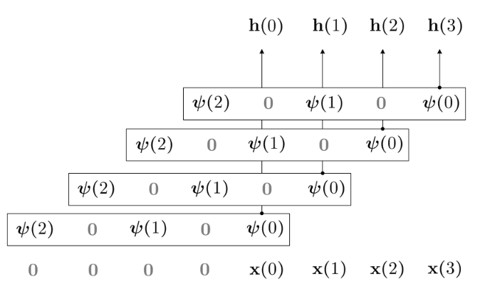
Visualization of Dilated Conv
This parameterization create its own limitations:
- Assumes no dependency on input values falling in the interleaved regions
Some work choose dilation factors in different layer carefully, to ensure each input is proceed by some kernel. However, this approach also has its own limitations:
- The resulting network is spare and it is hard to estimate how many linear/non-linear transformations are applied to each input
- This approach locks kernel_size, depth, dialiation_factor together, limiting the flexibility of network design
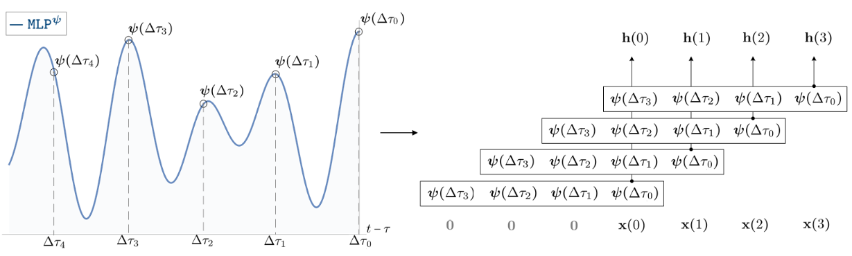
Continuous Kernel Convolution (CKConv)
Definition
Let $\psi$ be a convolutional kernel parameterized by a small neural network $\text{MLP}^\psi: \mathbb{R} \to \mathbb{R}^{N_{\text{out}} \times N_{\text{in}}}$
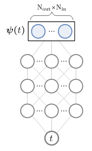
CKConv parameterized by a small neural network.
Following the theoretical framework, the authors define CKConv as:
\[(x * \psi)(t) = \sum_{c=1}^{N_{\text{in}}} \sum_{\tau=0}^t x_c(\tau) \text{MLP}_c^\psi (t-\tau)\]This representation is a bit problematic when then kernel size $N_K < t$:
\[(x * \psi)(t) = \sum_{c=1}^{N_{\text{in}}} \sum_{\tau=0}^{N_K} x_c(\tau) \text{MLP}_c^\psi (t-\tau)\]As you can see $x_c$ admit the time window $[0, N_K]$ instead of $[t-N_K, t]$.
I think an alternative definition is more interpretable for CS professionals (Similar swap also occurs in Appendix A.3, Equation 14):
\[(x * \psi)(t) = \sum_{c=1}^{N_{\text{in}}} \sum_{\tau=0}^t x_c(t-\tau) \text{MLP}_c^\psi (\tau)\]Where
\[\text{MLP}_c^\psi \in \mathbb{N_{\text{out}}}\]$x_c(t-\tau) \text{MLP}_c^\psi (\tau)$ maps the $c$-th dimension of $x(t-\tau)$ to some \(N_{\text{out}}\)-dimensional embedding.
This \(N_{\text{out}}\)-dimensional embedding is first sum across the time-dimension $\tau$, then sum across channel-dimension of $c$.
Properties
Arbitrarily Large Receptive Field
$\text{MLP}^\psi$ accepts relative time $t-\tau$ as input and returns the value of a convolutional kernel $\psi(t-\tau)$. Therefore, the kernel across equally space $N_K$ time step $(t-N_K\tau, …, t-2\tau, t-\tau, t)$ is:
\[\mathcal{K} = \{ \psi(\tau) \}_{\tau=0}^{N_K}\]To model long term dependency, increase the length $N_K$.
Irregularly Sampled Data
CKConvs can handle irregularly-sampled or partially observed data, due to kernel $\text{MLP}^\psi$ can be sampled at arbitrary positions $\tau$.
However, very non-uniformly / systematically imbalanced data will cause biased estimation. To overcome this, add a inverse sample density adjustment $s(\tau) = \frac{1}{p(\tau)}$:
\[(x * \psi)(t) = \int_{\mathbb{R}} s(t-\tau)x(t-\tau)\psi(\tau) d\tau\]Different Resolutions
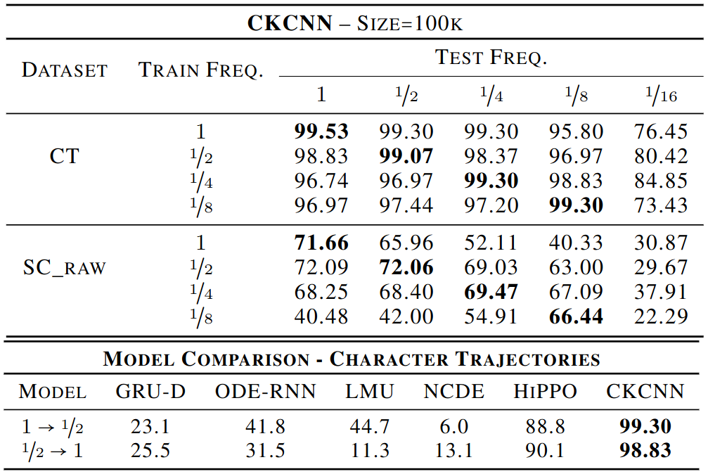
Suppose the kernel $(x * \psi)_{\text{sr1}}$ is trained at sampling rate sr1. To perform inference at sr2:
Reason: a Riemann integral defined on a finite grid at sampling rate sr is
where $\Delta_{\text{sr}} = \frac{1}{\text{sr}}$.
Then, we have:
\[\begin{align} \sum_{i=1}^{N_2} f(\tau_{2, i}) \Delta_2 \approx \sum_{i=1}^{N_1} f(\tau_{1, i}) \Delta_1 \\ \sum_{i=1}^{N_2} f(\tau_{2, i}) \frac{1}{\text{sr}_2} \approx \sum_{i=1}^{N_1} f(\tau_{1, i}) \frac{1}{\text{sr}_1} \\ (x * \psi)_{\text{sr2}}(t) \approx \frac{\text{sr}_2}{\text{sr}_1} (x * \psi)_{\text{sr1}}(t) \end{align}\]Connection to Linear Recurrent Unit
Consider a linear recurrent unit unrolled for $t$ steps:
\[h(t) = W^{t+1} h(-1) + \sum_{\tau=0}^t W^\tau U x(t-\tau)\]where $h(-1)$ is the initial hidden state.
The corresponding convolution output, signal $x$ and kernel $\psi$ are:
\[x = [x(0), x(1), ..., x(t-1), x(t)] \psi = [U, WU, ..., W^{t-1}uU, W^t U] h(t) = \sum_{\tau=0}^t x(t-\tau)\psi(\tau)\]The exploding and vanishing gradients in RNN occurs when the eigenvalue of $W$ not equals to $1$.
The kernel $\psi = [U, WU, …, W^{t-1}uU, W^t U]$ implies that Linear recurrent units can be described as a convolution between the input and a very specific class of convolutional kernels: exponential functions. However, convolutional kernels are not restricted to exponential functional class, indicating that CKConv is more flexible than RNN.
Parameterization
CKConv relies on the assumption that the neural network $\text{MLP}^\psi$ is able to model complex dependencies or generate arbitrary convolutional kernels.
We need to verify this assumption for different MLP parameterization, e.g., with different piece-wise activation functions: ReLU, LeakyReLU and Swish.
Connection to Implicit Neural Representation
- [Occupancy networks: Learning 3d reconstruction in function space, CVPR 2019]
- [Deepsdf: Learning continuous signed distance functions for shape representation, CVPR 2019]
- [Implicit neural representations with periodic activation functions, NIPS 2020]
Implicit neural representations study generic ways to represent low-dimensional (e.g., $\mathbb{R}^2$) data, via neural networks.
A concrete example is: given a $256 \times 256$ image, train a neural network to learn the mapping $\phi$ from $(x_1,x_2)$ coordinate to RGB-tuple $(y_1,y_2, y_3)$. This allows us to work with the image in a more analytical and differentiable manner. For example, the image is discrete, assume the underlying generating function of the image is continuous and we can learn this continuous mapping by $\phi$. Then we can perform tasks like: changing colors, morphing shapes, super-resolution or compression.
In case of convolutional kernel estimation, note that the below 2 are almost equivalent:
- Parameterizing a convolutional kernel with a neural network
- Constructing an implicit neural representation of the kernel
With the subtle difference: for CKConv, the target of implicit neural representation is not known a-priori, but learned as part of the optimization.
Recent works in Implicit Neural Representation found that MLP with piece-wise activation functions are unable to model high-frequencies data (which is quite common in certain types of sequence data). Random Fourier features and Sine nonlinearities yields better results.
CKConvs with SIREN Kernels
SIREN, or MLP with Sine nonlinearities, is defined as follow:
\[y = \text{Sine}(\omega_0 [Wx + b])\]where $\omega_0$ is non-learnable and serves as a prior for the oscillations of the output.
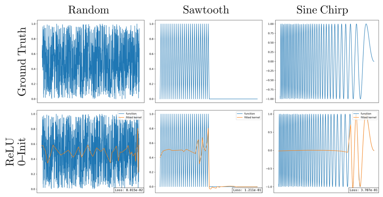
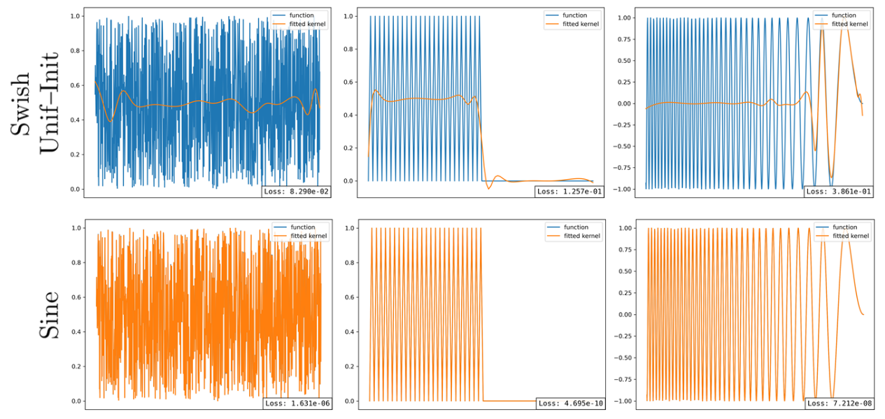
Function approximation via ReLU, Swish and Sine networks. For non-linear, non-smooth functions, only Sine provide good approximations.
The empirical result shows that CKConvs with SIREN kernels have the ability to model complex input dependencies across large memory horizons.
Experiments
Architecture
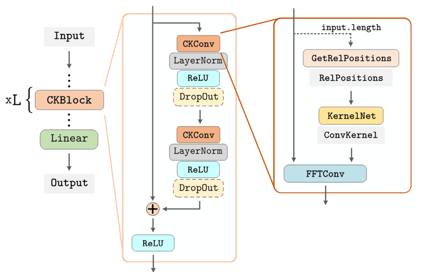
Dot-lined blocks depict optional blocks, and blocks without borders depict variables. KernelNet blocks use Sine nonlinearities. We replace spatial convolutions by Fourier Convolutions (FFTConv), which leverages the convolution theorem to speed up computations.
Convolutional kernels: 3-layer SIRENs
Vector-valued 3-layer neural network with 32 hidden units and Sine nonlinearities:
\[1 \to 32 \to 32 \to N_{\text{out}} \times N_{\text{in}}\]where $N_{\text{out}}, N_{\text{in}}$ are number of input and output channels
Normalized relative positions
Map the largest unitary step-wise relative positions seen during training $[0,N]$ to a uniform linear space in $[−1, 1]$ to maintain numerical stability.
Other Architecture details
- Weight normalization (faster convergence)
- [Weight normalization: A simple reparameterization to accelerate training of deep neural networks, 2016]
- FFTConv to speed up the convolution
Hyperparameter
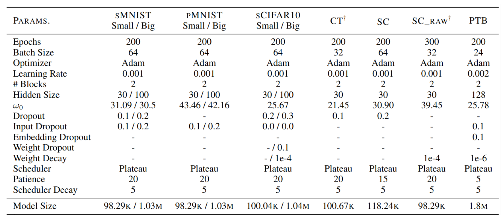
Hyperparameter of the best performing CKCNN models. CKCNN is sensitive to $\omega_0$.
Selection of $\omega_0$
CKCNNs are very sensitive to $\omega_0$. Random search is performed on a large interval $\omega_0 \in [0, 3000]$
Tasks
- pMNIST: performance vary from 98.54 to 65.22 for values of $\omega_0$ in [1, 100].
- Copy Memory: optimal $\omega_0$ found are 19.20, 34.71, 68.69, 43.65 and 69.97 for the corresponding sequence lengths.
- Adding Problem: optimal $\omega_0$ found are 14.55, 18.19, 2.03, 2.23 and 4.3 for the corresponding sequence lengths.
Copy Memory and Adding Problem
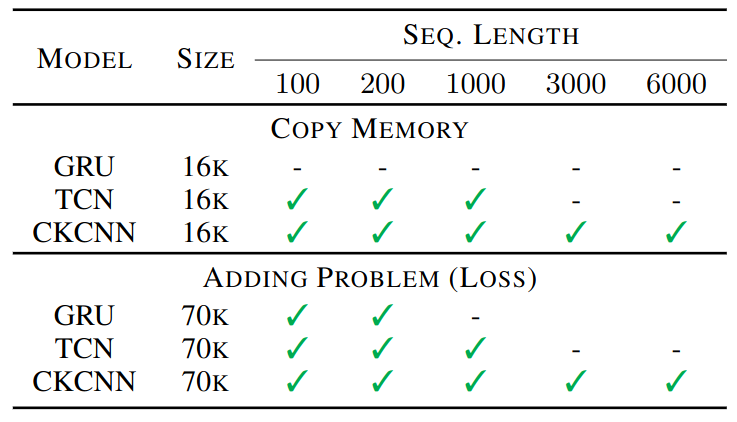
A shallow CKCNN can solve both problems for all sequence lengths. GRU and TCN (with k=7, n=7) struggle to solve both.
Discrete sequential datasets
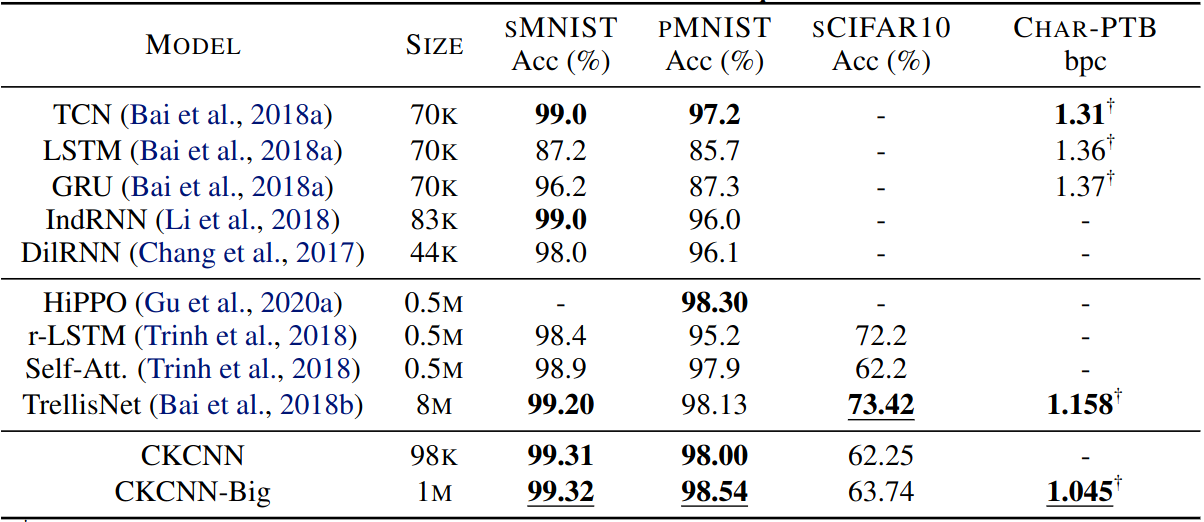
Shallow CKCNNs is SOTA competitive using 5x-80x fewer parameters.
Author report CKCNN heavily overfitted sCIFAR10. Combinations of weight decay, dropout and weight dropout were not enough to counteract overfitting.
Speech Commands (SC)
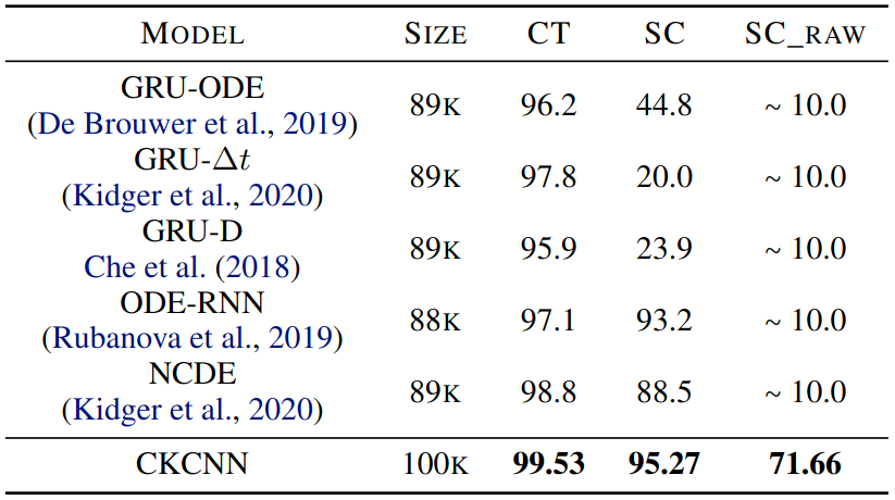
Personal thought: this is not a fair comparison, should consider TCN-RNN models.
Author report that, on SC, high-frequency component hurt performance when performing super resolution.
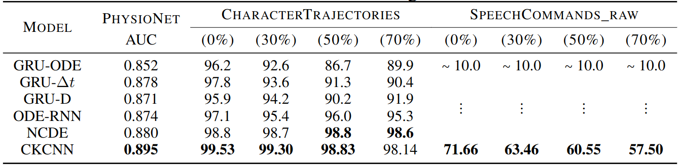
Irregularly Sampled Data
Different Resolutions