Conditioned-RLFT
This post is mainly based on
C-RLFT vs DPO vs RLHF
- RLHF: requires preference data, requires training a reward model
- DPO: requires preference data
- C-RLFT: requires mixed-quality data from different sources, does not require preference labels
C-RLFT
- Fine-tune LLM with mixed quality training data
- A small amount of expert data
- A large proportion of sub-optimal data
- No preference label required
- C-RLFT
- Learn a class-conditioned policy using coarse-grained reward labels (e.g., data sources: GPT-4 vs GPT-3.5)
- The learned policy contains latent data quality information
- Optimal policy can be solved through single-stage, RL-free supervised learning
- Results
- openchat-13b outperforms SOTA open-source 13B model
Background
Given a conversation dataset $D = \{ (x_i, y_i) \}$ and a pre-trained LLM $\pi_0 (y | x)$. Goal: learn an optimal policy that maximize some loss function $J(\theta | D)$.
Supervised Fine-tuning (SFT)
Directly optimize $\pi_\theta$ via MLE:
\[J_{\text{SFT}}(\theta) = \mathbb{E}_{(x,y) \sim D} [\log \pi_\theta (y|x)]\]Problem: if the training dataset $D$ is mixed quality, the low-quality data are likely to negatively impact learning.
Reinforcement Learning Fine-tuning (RLFT)
Requires a reward model $r(x,y)$, either explicitly or implicitly.
KL-regularized RL
- A popular RL framework for fine-tuning LLMs
- Adds an additional KL penalty to constrain $\pi_\theta(y|x)$ to stay close to $\pi_0(y|x)$
- Avoid distribution collapse as compared to naively maximize reward using RL
- Paper
- [Way off-policy batch deep reinforcement learning of implicit human preferences in dialog, 2019]
- [RL with KL penalties is better viewed as Bayesian inference, EMNLP 2022]
Problem: requires collecting considerable amounts of costly pairwise (or ranking-based) human preference feedback.
C-RLFT
Learn optimal policy from $D_{\text{exp}} \cup D_{\text{sub}}$, where the quality difference between expert demonstration $D_{\text{exp}}$ and suboptimal dataset $D_{\text{sub}}$ itself serve as implicit/weak reward signals.
Regularizing $\pi_\theta$ with a better and more informative class-conditioned reference policy $\pi_C$ instead of the pre-trained LLM $\pi_0$.
Class-Conditioned Dataset and Reward
Construct a class conditioned dataset $D_c = {(x_i, y_i, c_i)}$.
$c_i$ is class labels and $c_i \in {\text{GPT-4}, \text{GPT-3.5}}$.
Let $\pi_c(y | x,c)$ be a class-conditioned policy.
Encode coarse-grained rewards $r_c(x, y)$ in $D_c$ as:
\[r_c(x_i, y_i) = \begin{cases} 1, & \text{if } (x_i, y_i) \in D_{\text{exp}} \quad (c_i = \text{GPT-4}), \\ \alpha, & \text{if } (x_i, y_i) \in D_{\text{sub}} \quad (c_i = \text{GPT-3.5}) \end{cases}\]Set $\alpha < 1$ to guide $\pi_\theta$ to favor GPT-4’s responses.
C-RLFT
Class-Conditioned Policy
To create the class-condition $c$, we can condition examples from each data source with a unique initial prompt:
$c_i = \text{GPT-4}$:
GPT4 User: Question<|end of turn|>GPT4 Assistant:
$c_i = \text{GPT-3.5}$:
GPT3 User: Question<|end of turn|>GPT3 Assistant:
A new <|end of turn|> special token is introduced to stop generation while preventing confusion with the learned meaning of EOS during pretraining.
Policy Optimization
\[J_{\text{C-RLFT}}(\theta) = \mathbb{E}_{y \sim \pi_\theta} [r_c(x,y)] - \beta D_{\text{KL}}(\pi_\theta, \pi_c)\]The loss function induced 2 optimization goals:
- Maximize reward
- Equivalent to optimize the policy to generate distribution from expert dataset
- Regularization
- Regularize $\pi_\theta$ w.r.t reference policy $\pi_c$ instead of pre-trained model $\pi_0$
- Note that we do not need to explicitly solve for $\pi_c$, as it will merge into our sampling procedure from $D_c$ in [Eq 6]
It can be shown that the optimal solution to the above loss is:
[Eq 5]
\[\pi^*(y|x,c) \propto \exp\left( \frac{1}{\beta} r_c(x,y) \right) \pi_c(y|x,c)\]where $\exp\left( \frac{1}{\beta} r_c(x,y) \right)$ can be viewed a weight of a reference policy
- $r_c$ control the preference over a dataset
- $\beta$ control the sharpness/uniformity of the weight distribution
Now we have obtained $\pi^*$.
Using a few tricks in [Eq 6], we can optimize $\pi_\theta$ toward $\pi^*$:
[Eq 6]
\[\begin{align} \pi_\theta &= \text{argmin}_\theta \mathbb{E}_{(x,c) \sim D_c}\left[ D_{KL}( \pi^*(\cdot|x,c) \| \pi_\theta(\cdot|x,c) ) \right] \\ &= \text{argmin}_\theta \mathbb{E}_{(x,c) \sim D_c}\left[ \mathbb{E}_{y \sim \pi^*}[ -\log \pi_\theta (y|x,c) ] \right] \\ &= \text{argmax}_\theta \mathbb{E}_{(x,y,c) \sim D_c}\left[ \exp\left( \frac{1}{\beta} r_c(x,y) \right) \log \pi_\theta (y|x,c) \right] \end{align}\]1st to 2nd line:
\[D_{KL}( P \| Q ) = \sum_{x \in X} P(x) \log( \frac{P(x)}{Q(x)} ) = -\sum_{x \in X} P(x) \log( \frac{Q(x)}{P(x)} )\]Since $P(x)$ is $\pi^*$, which is independent of $\theta$, $P(x)$ can be treated as a constant. Due to we are optimizing for $\text{argmin}_\theta$ and a constant does not affect the result, we can ignore this constant term. This results in:
\[D_{KL}( \pi^*(\cdot|x,c) \| \pi_\theta(\cdot|x,c) ) \propto \sum \pi^*(y|x,c) [ -\log \pi_\theta(\cdot|x,c) ]\]Due to sampling from a distribution is equivalent to a weighted sum of the distribution.
\[\sum \pi^*(y|x,c) [ -\log \pi_\theta(\cdot|x,c) ] = \mathbb{E}_{y \sim \pi^*}[-\log \pi_\theta(\cdot|x,c)]\]2nd to 3rd line:
Substitute the optimal policy [Eq 5], we have
\[\mathbb{E}_{y \sim \pi^*}[ \log \pi_\theta (y|x,c) ] \propto \mathbb{E}_{y \sim \pi_c} \left[ \exp\left( \frac{1}{\beta} r_c(x,y) \right) \log \pi_\theta (y|x,c) \right]\]Note that merging 2 sampling procedure \(\mathbb{E}_{(x,c) \sim D_c}\) and \(\mathbb{E}_{y \sim \pi_c}\) together, is equivalent to directly sampling from the $D_c$ dataset:
\[\mathbb{E}_{(x,c) \sim D_c}[\mathbb{E}_{y \sim \pi_c} f(\theta) ] = \mathbb{E}_{(x,y,c) \sim D_c}[ f(\theta) ]\]This suggests that the fine-tuned policy $\pi_\theta$ can be learned through a simple reward-weighted regression objective with the class-conditioned dataset $D_c$.
Model Inference
Assuming model tuned under C-RLFT has learned to distinguish expert and sub-optimal data distributions.
Then prompt the model conditioned on the expert dataset to get expert response:
GPT4 User: Question<|end of turn|>GPT4 Assistant:
Experiments
- Data: ShareGPT conversations dataset following Vicuna
- 6k expert conversations generated by GPT-4
- 64k sub-optimal conversations generated by GPT-3.5
- Model: llama-2-13b as the base model
LLM Benchmarks
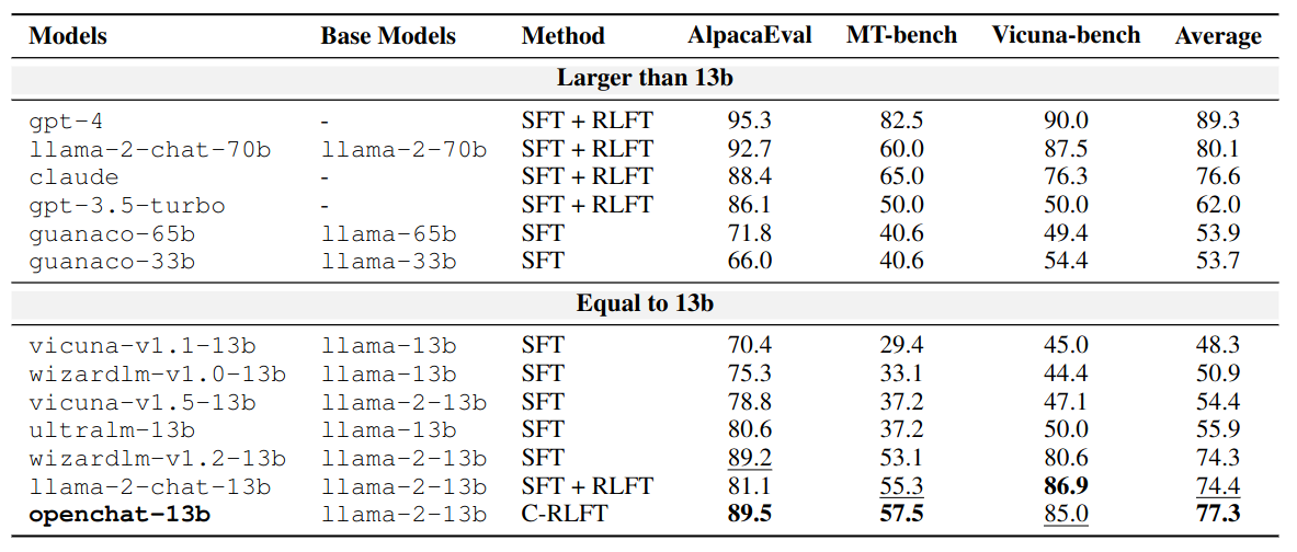
Win-rate (%) against: text-davinci-003 in AlpacaEval, and gpt-3.5-turbo in both MT-bench and Vicuna-bench.
Ablation Study
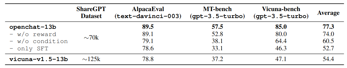
Ablation studies of coarse-grained rewards (reward) and class-conditioned policy (condition) to openchat-13b.
C-RLFT Analysis
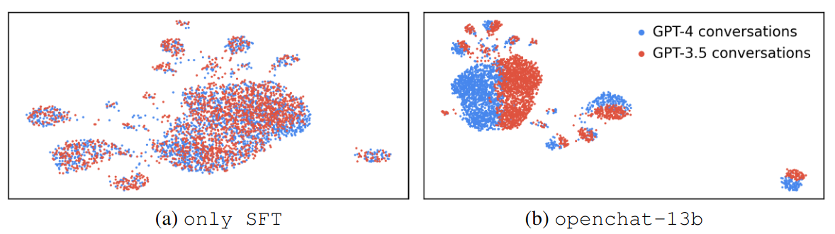
Visualization of GPT-4 and GPT-3.5 conversations’ representations. only SFT: GPT-3.5 and GPT-4 representations are intermingled; openchat-13b: GPT-3.5 and GPT-4 representations are clearly distinguished.
How to obtain this visualization?
- Embedding: mean pooling of all tokens in the last Transformer layer output
- Dimension reduction: UMAP to 2-D space
- Umap: Uniform manifold approximation and projection
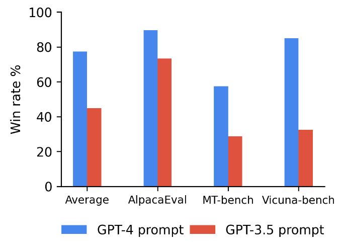
Effects of class-conditioned prompt tokens during inference phase. Substantial performance decline observed when using the GPT-3.5 prompt instead of the GPT-4 prompt.