Direct Preference Optimization

This post is mainly based on

• Direct Preference Optimization: Your Language Model is Secretly a Reward Model, NIPS 2023

RLHF vs DPO

• Assumption: human preference data is generated from some preference model
• RLHF
  • Use the preference model $p^*$ to define a preference loss $\mathcal{L}_P$, then train a reward model \(r_\phi\)
  • Based on reward model $r_\phi$, train a policy $\pi_\theta$ that maximize reward subject to some constraints
• DPO
  • Use a change of variables to define the preference loss as a function of the policy directly

Direct Preference Optimization

• Motivation: RLHF on large scale language model fine-tuning is hard
• DPO
  • Use a theoretical preference model (Bradley-Terry model) to measures how well a given reward function aligns with empirical preference data
  • Each DPO update increases the relative log probability of “win” to “loss” responses
  • Implicitly optimizes the same objective as RLHF
• Results
  • SOTA Competitive to RLHF with almost no hyperparameter tuning

Background

Bradley-Terry (BT) Model

• [Rank analysis of incomplete block designs: I. the method of paired comparisons, 1952]

probability that entity $A$ will win over entity $B$ in a pairwise comparison is given by the formula:

\[P(A>B) = \frac{ \exp(\beta_A) }{ \exp(\beta_A) + \exp(\beta_B) }\]

where $\beta_A, \beta_B$ are interpreted as the “strengths” or “skills” of the entities.

The Bradley-Terry model is widely used in various fields, including sports, psychology and machine learning (for ranking algorithms). It provides a straightforward way to estimate the relative strengths of entities based on comparison outcomes.

Contextual Dueling Bandit (CDB)

• Contextual dueling bandits, PMLR 2015
• Contextual bandit vs CDB
  • Contextual bandit learns by rewards
  • Contextual dueling bandit learns by preferences or rankings of actions
• Theoretical analysis of CDBs substitutes the notion of an optimal policy with a von Neumann winner, a policy whose expected win rate against any other policy is at least 50%.

CDB vs HF

• CDB: preference labels are given online
• Learning from Human Feedback: learn from a fixed batch of offline preference-annotated action pairs

Preference-based RL (PbRL)

Learns from binary preferences generated by an unknown “scoring” function rather than rewards.

Existing methods generally involve first explicitly estimating the latent scoring function (i.e. the reward model) and subsequently optimizing it.

PbRL papers

• [Preference-based reinforcement learning: evolutionary direct policy search using a preference-based racing algorithm, 2014]
• [Dueling rl: Reinforcement learning with trajectory preferences, PMLR 2023]
• [Deep reinforcement learning from human preferences, NIPS 2017]
• [Active preference-based learning of reward functions, 2017]

RLHF

Supervised fine-tuning (SFT)

Supervised learning produce: $\pi^{\text{SFT}}$

Reward Modelling

First, prompt the supervised model $\pi^{\text{SFT}}$ with $x$ to obtain an answer pair $(y_1, y_2) \sim \pi^{\text{SFT}} (y | x)$.

Then, human labeler express preference: $y_w \succ y_l | x$. The preferences are assumed to be generated by some latent reward model $r^*(y, x)$, which we do not have access to.

The human preference distribution $p^*$ under BT model can be written as:

\[p^*(y_1 \succ y_2 | x) = \frac{\exp(r^*(x, y_1))}{\exp(r^*(x, y_1)) + \exp(r^*(x, y_2))}\]

Above is a preference model and it could be viewed as a binary classification problem.

We can parametrize a reward model $r_\phi(x, y)$ and estimate the parameters $\phi$ via maximum likelihood.

To learn $\phi$, we need a loss function:

\[\mathcal{L}_P(r_\phi, D) = -\mathbb{E}_{(x,y_u,y_l) \sim D} \left[ \log \sigma (r_\phi (x, y_u) - r_\phi (x, y_l)) \right]\]

where

• $\mathcal{L}_P$ is a preference loss
• $D$ is the dataset of pairwise data $ D = { x, y_w, y_l } $ sampled from $p^*$
• $\sigma$ is logistic function

$r_\phi(x, y)$ is often initialized from $\pi^{\text{SFT}}(y | x)$ with a linear layer on top of the transformer layer to project the embedding to a scalar reward value.

To ensure a reward function with lower variance, prior works normalize the rewards:

\[\mathbb{E}_{x,y \sim D} [r_\phi(x, y)] = 0\]

RL Fine-Tuning

[Eq 3] Optimize the language model policy to maximize the reward:

\[\max_{\pi_\theta} \mathbb{E}_{x \sim D, y \sim \pi_\theta(y | x)} [ r_\phi (x, y) ] - \beta \mathbb{D}_{\text{KL}} [ \pi_\theta(y | x) || \pi_{\text{ref}}(y | x) ]\]

where

• $\pi_{\text{ref}}$ is the reference policy used to regulate the loss
• $\beta$ is regularization parameter
• $\pi_\theta$ is often initialized to $\pi_{\text{SFT}}$

Due to the policy $\pi_\theta$ output discrete tokens, the above loss is not differentiable and is typically optimized with reinforcement learning.

The reward function is typically constrcuted as follow:

\[r(x, y) = r_\phi (x, y) - \beta ( \log \pi_\theta(y | x) - \log \pi_{\text{ref}}(y | x) )\]

RLHF papers

• Fine-Tuning Language Models from Human Preferences, 2019
• Learning to summarize from human feedback, 2022
• Training a helpful and harmless assistant with reinforcement learning from human feedback, 2022
• [Training language models to follow instructions with human feedback, NIPS 2022]

Direct Preference Optimization (DPO)

Given a dataset of human preferences over model responses, DPO optimize a policy using a simple binary cross entropy objective, producing the optimal policy to an implicit reward function fit to the preference data.

Key Insight

• There is an analytical mapping from reward functions $r$ to optimal policies $\pi^*$
• With this mapping, we can transform a loss function over $r$ into a loss function over $\pi$
• This change-of-variables approach can:
  • Avoids fitting an explicit, standalone reward model
  • While still optimizing under existing models of human preferences (e.g., Bradley-Terry model)
• The authors show that the policy network represents both:
  • The language model
  • The (implicit) reward

Deriving the DPO objective

Claim optimal solution to [Eq 3] is (derivation see paper’s Appendix A.1):

\[\pi_r(y | x) = \frac{1}{Z(x)} \pi_{\text{ref}}(y | x) \exp \left( \frac{1}{\beta} r(x, y) \right)\]

where $Z(x)$ is the partition function:

\[Z(x) = \sum_y \pi_{\text{ref}}(y | x) \exp \left( \frac{1}{\beta} r(x, y) \right)\]

The problem with the above solution is: $Z(x)$ is intractable and hard to estimate. However, we can rearrange the terms w.r.t. $r(x, y)$:

\[r(x, y) = \beta \log\frac{\pi_r(y | x)}{\pi_{\text{ref}}(y | x)} + \beta \log Z(x)\]

The Bradley-Terry model can be rewritten as:

\[\begin{align} p^*(y_1 \succ y_2 | x) &= \frac{\exp(r^*(x, y_1))}{\exp(r^*(x, y_1)) + \exp(r^*(x, y_2))} \\ &= \frac{1}{1 + \frac{\exp(r^*(x, y_2))}{\exp(r^*(x, y_1))} } \\ &= \frac{1}{1 + \exp(r^*(x, y_2) - r^*(x, y_1)) } \\ &= \sigma(r^*(x, y_1) - r^*(x, y_2)) \end{align}\]

Due to $\sigma(z) = \frac{1}{1+\exp(-z)}$. The interpretation is: Bradley-Terry model depends only on the difference of rewards between two completions $y_1$ and $y_2$.

Substitute $r(x, y)$ into the above equation, we have:

\[p^*(y_1 \succ y_2 | x) = \sigma \left( \beta \log\frac{\pi^*(y_1 | x)}{\pi_{\text{ref}}(y_1 | x)} - \beta \log\frac{\pi^*(y_2 | x)}{\pi_{\text{ref}}(y_2 | x)} \right)\]

where the intractable $\beta \log Z(x)$ cancel each other. There is also a equation for the more general Plackett-Luce models, shown in paper’s Appendix A.3.

Note that this yields the expression of probability of human preference $p^(y_1 \succ y_2 | x)$ in terms of the optimal policy $\pi^$ rather than the reward model $r^*(x,y)$. We can write an MLE loss for optimization as follow:

[Eq 7]

\[\begin{align} \mathcal{L}_{\text{DPI}}(\pi_\theta; \pi_{\text{ref}}) &= -\mathbb{E}_{x, y_w, y_l \sim D} \left[ \log\sigma \left( \beta \log\frac{\pi_\theta(y_w | x)}{\pi_{\text{ref}}(y_w | x)} - \beta \log\frac{\pi_\theta(y_l | x)}{\pi_{\text{ref}}(y_l | x)} \right) \right] \\ &= -\mathbb{E}_{x, y_w, y_l \sim D} \left[ \log\sigma ( \hat{r}_\theta(x, y_w) - \hat{r}_\theta(x, y_l) ) \right] \end{align}\]

where \(\hat{r}_\theta(x, y) = \beta \log\frac{\pi_\theta(y \| x)}{\pi_{\text{ref}}(y \| x)}\)

Since this procedure is equivalent to fitting a reparametrized Bradley-Terry model, it enjoys certain theoretical properties, such as consistencies under suitable assumption of the preference data distribution.

What does the DPO update do?

Taking gradient from [Eq 7] w.r.t. to $\theta$ yields:

\[\nabla_\theta \mathcal{L}_{\text{DPI}}(\pi_\theta; \pi_{\text{ref}}) = -\beta\mathbb{E}_{x, y_w, y_l \sim D} \left[ \text{TERM 1} ( \text{TERM 2} - \text{TERM 3} ) \right]\]

where

TERM 1 = \(\sigma( \hat{r}_\theta(x, y_l) - \hat{r}_\theta(x, y_w) )\) and will assign higher weight when reward estimate is wrong

TERM 2 = \(\nabla_\theta \log \pi(y_w \| x)\), each update increase likelihood of $y_w$

TERM 3 = \(\nabla_\theta \log \pi(y_l \| x)\), each update decrease likelihood of $y_l$

DPO workflow

Step 1. Sample completions $y_1, y_2 \sim \pi_{\text{ref}}( \cdot | x )$ for every prompt $x$, label with human preferences to construct an offline dataset $D$.

Step 2. Optimize the language model $\pi_\theta$ to minimize $\mathcal{L}_{\text{DPO}}$, given

• The completion generator policy $\pi_{\text{ref}}$
• The offline dataset $D$
• $\beta$

In practice, we usually reuse public preference dataset generated with $\pi^{\text{SFT}}$ and attempt to initialize $\pi_{\text{ref}} = \pi^{\text{SFT}}$

Theoretical Analysis of DPO

TBD

Experiments

Questions to answer

• Q1: How efficiently does DPO trade off maximizing reward and minimizing KL-divergence with the reference policy, compared to common preference learning algorithms such as PPO?
• Q2: How does DPO perform on larger models and more difficult RLHF tasks, including summarization and dialogue?

Methods

• [TBD]

Controlled sentiment generation

• Data
  • $x$: a prefix of a movie review from the IMDb dataset
  • $y$: positive sentiment completion of $x$ generated by some policy
  • Preference pairs are generated by a pre-trained sentiment classifier $p(\text{positive} | x, y)$
• SFT model: fine-tune GPT-2-large until convergence on reviews from the train split of the IMDB dataset
• Evaluation
  • Under same KL discrepancy, how much reward a model can achieve
  • Train multiple models with different hyperparameters to induce different policy conservativeness

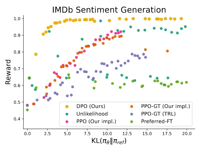
Reward-KL frontier for various algorithms in the sentiment setting. DPO produces by far the most efficient frontier.

Summarization

• Data
  • $x$: a forum post from Reddit TL;DR summarization dataset
  • $y$: summary $y$ of the main points in the post generated by some policy
  • Preference pairs are gathered by Stiennon et al
• SFT model: fine-tuned on human-written forum post summaries with the TRLX framework for RLHF
• Evaluation
  • Sampling completions on the test split of TL;DR summarization dataset
  • Compute win rates vs. test split’s human-written summaries, using GPT-4 as evaluator

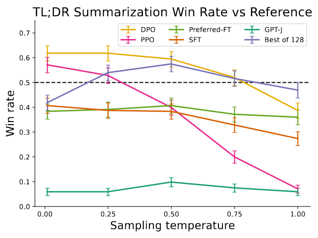
DPO exceeds PPO’s performance, while being more robust to changes in the sampling temperature.

zero-shot prompting with GPT-J

Single-turn dialogue

• Data
  • $x$: a human query, which may be anything from a question about astrophysics to a request for relationship advice
  • $y$: an engaging and helpful response to query $x$, generated by some policy
  • Anthropic Helpful and Harmless dialogue dataset (Anthropic HH): 170k dialogues between a human and an automated assistant. Each transcript ends with a pair of responses generated by LLM + a preference label
• SFT model: No pre-trained SFT model is available. The author fine-tune an off-the-shelf language model on only the preferred completions to form the SFT model
• Evaluation
  • Sampling completions on the test split of Anthropic HH
  • Compute win rates vs. test split’s preferred completions, using GPT-4 as evaluator

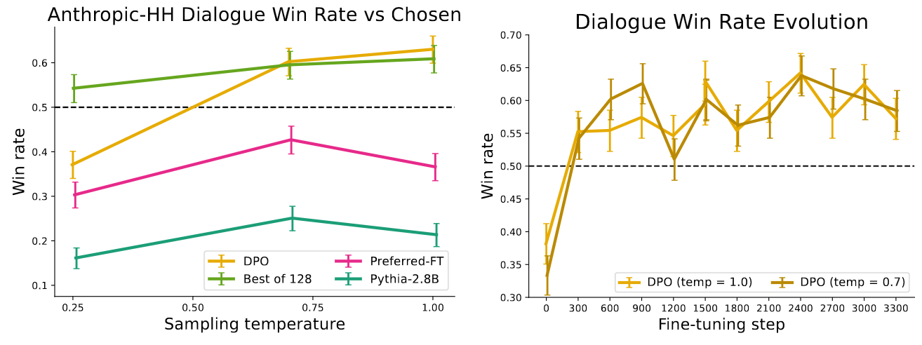
Left: DPO’s win rate dialogue task. Right: DPO converges to its best performance relatively quickly.

Robustness under Distribution Shift

• Train on: Reddit TL;DR summarization dataset
• Evaluate on: test split of the CNN/DailyMail dataset

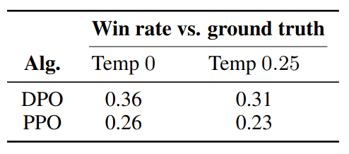
GPT-4 win rates vs. ground truth summaries for out-of-distribution CNN/DailyMail input articles.