Mamba: Selective State Space Model
This post is mainly based on
Mamba
- Motivation
- SSM does not performed as well as attention on important modalities such as language
- Key weakness of SSM: inability to perform content-based reasoning
- Improvements
- Letting the SSM parameters be functions of the input allowing the model to selectively propagate or forget information along the sequence length dimension, depending on the current token
- The above change prevents the use of efficient convolutions, therefore a hardware-aware parallel algorithm in recurrent mode is designed
- Mamba
- Fast inference (5x higher throughput than Transformers)
- Linear scaling in sequence length
- Performance improves on real data up to million-length sequences
- Mamba-3B model outperforms Transformers of the same size and matches Transformers twice its size, both in pretraining and downstream evaluation
The efficacy of self-attention is attributed to its ability to route information densely within a context window, allowing it to model complex data. However, self-attention also has drawbacks:
- Inability to model anything outside of a finite window
- Quadratic scaling with respect to the window length
Selection Mechanism
- Identify a key limitation of prior models: the ability to efficiently select data in an input-dependent manner (i.e. focus on or ignore particular inputs)
- Design a simple selection mechanism by parameterizing the SSM parameters based on the input
- Allows the model to filter out irrelevant information and remember relevant information indefinitely
Hardware-aware Algorithm
- The Selection Mechanism poses a technical challenge for the computation
- Hardware-aware algorithm
- Computes the model recurrently with a scan instead of convolution
- Does not materialize the expanded state in order to avoid IO access between different levels of the GPU memory hierarchy
- Result: faster than previous methods
- In theory: scaling linearly in sequence length, compared to pseudo-linear for all convolution-based SSMs
- On modern hardware: up to 3x faster on A100 GPUs
Architecture
- Mamba: fully recurrent models
- Suitable as the backbone of foundation models operating on sequences
- High quality: selectivity brings strong performance on dense modalities such as language and genomics
- Fast training and inference
- Computation and memory scales linearly in sequence length during training
- Unrolling the model autoregressively during inference requires only constant time per step
- Long context: the quality and efficiency together yield performance improvements on real data up to sequence length 1M
Benchmarks
- Synthetics
- Tasks: copying and induction heads
- Mamba solves the tasks easily but can extrapolate solutions indefinitely long (>1M tokens)
- Audio and Genomics
- Out-performs SOTA models (SaShiMi, Hyena, Transformers) on modeling audio waveforms and DNA sequences
- Performance improves with longer context up to million-length sequences
- Language Modeling
- First linear-time sequence model that truly achieves Transformer-quality performance
- Scaling up to 1B parameters, Mamba exceeds the performance of a large range of baselines
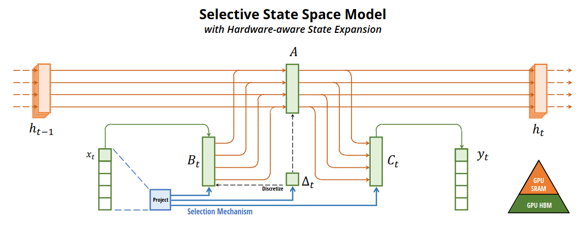
Structured SSMs
- From: input $x$, with dimension $D=5$
- Map each dimension to latent state $h$, with dimension $N=4$ (Total 20 dim for $D=5$ input)
- The mapping is parametrized by $(\Delta, A, B, C)$
- $A$: similar to input gate
- $B$: similar to forget gate
- $C$: similar to output gate / directly input dependent
- $\Delta$: step size of the discretization / modulates model dependencies length $\frac{1}{\Delta}$
- To: output $y$, with some output dimension
State Space Model
Structured State Space Sequence Models (S4)
S4 models are parameterized by: $(\Delta, A, B, C)$, with continuous representation:
\[\begin{align} h'(t) &= Ah(t) + Bx(t) \\ y(t) &= Ch(t) \end{align}\]Recurrent representation:
\[\begin{align} h_t &= \bar{A}h_{t-1} + \bar{B}x_t \\ y_t &= Ch_t \end{align}\]Convolutional representation:
\[\begin{align} \bar{K} &= (C\bar{B}, C\bar{A}\bar{B}, ..., C\bar{A}^k\bar{B}, ...) \\ y &= x * \bar{K} \end{align}\]Discretization
Transforms the “continuous parameters” $(\Delta, A, B)$ to “discrete parameters” $(A, B)$
There are many discretization rule. For example, zero-order hold (ZOH):
\[\begin{align} \bar{A} &= \exp(\Delta A) \\ \bar{B} &= (\Delta A)^{-1}( \exp(\Delta A) - I) \cdot \Delta B \end{align}\]Discretization has deep connections to continuous-time systems. This equip them with useful properties:
- Resolution invariance
- Automatically ensuring that the model is properly normalized
- Connections to gating mechanisms of RNNs
Linear Time Invariance (LTI)
- LTI
- Model’s dynamics are constant through time
- $(\Delta, A, B, C)$ or $(\bar{A}, \bar{B})$ are fixed across all time-steps
- LTI is deeply connected to recurrence and convolutions
- To date, all structured SSMs have been LTI (For efficient training in convolution mode)
- However, LTI models have fundamental limitations in modeling certain types of data
- This paper’s technical contributions involve
- Removing the LTI constraint
- Overcoming the efficiency bottlenecks
Structure and Dimensions
- Structured SSMs
- “Structured” due to SSM requires imposing structure on the $A$
- Special structure on $A$ ensures that convolution can be computed efficiently
- Example: diagonal $A$ for diagonal state space model
- Efficiency bottleneck
- Assume
- Input $x$ is $D$ dimensional
- Batch size $B$
- Sequence length $L$
- Hidden state $h$, with hidden state dimension $N$
- Total hidden state has dimension $ND$
- Total compute and memory: $O(BLDN)$
- This is the fundamental efficiency bottleneck
- Assume
SSM Architectures
- SSM is referred to as SSNN, (similar to linear convolution layers are called CNNs)
- Linear attention
- Approximation of self-attention involving a recurrence
- Can be viewed as a degenerate linear SSM
- H3
- S4 based
- Can be viewed as an SSM sandwiched by two gated connections
- A shift-SSM, before the main SSM layer
- Hyena
- Same as H3 but replaces the S4 layer with an MLP-parameterized global convolution
- RetNet
- Adds an additional gate to the architecture
- Uses a simpler SSM
- Uses a variant of multi-head attention (MHA) instead of convolutions
- RWKV
- Another linear attention approximation
- Its main “WKV” mechanism involves LTI recurrences and can be viewed as the ratio of two SSMs
S5, QRNN, and SRU are the most closely related methods to selective SSM
- QRNN: [Quasi-recurrent Neural Networks, 2016]
- SRU: [Simple Recurrent Units for Highly Parallelizable Recurrence, 2017]
- SRU++: [When Attention Meets Fast Recurrence: Training Language Models with Reduced Compute, 2021]
Selective State Space Models
Motivation
- Fundamental problem of sequence modeling
- How to compress context into a smaller state?
- Popular sequence models could be viewed as tradeoffs on level of compression
- Attention
- Does not compress context at all
- Autoregressive inference requires explicitly storing the entire context (i.e. the KV cache)
- Directly causes the slow linear-time inference and quadratic-time training of Transformers
- Recurrent models
- Finite state: constant-time inference and linear-time training
- Effectiveness is limited, due to context is not well compressed into the state
Synthetic tasks
- Selective Copying Task
- Modifies the Copying task: position of the tokens to be memorized is changed
- Requires content-aware reasoning to be able to:
- Memorize the relevant tokens (colored)
- Filter out the irrelevant ones (white)
- Induction Heads Task
- A well-known mechanism hypothesized to explain the majority of in-context learning abilities of LLMs
- Requires context-aware reasoning to know when to produce the correct output in the appropriate context (black)
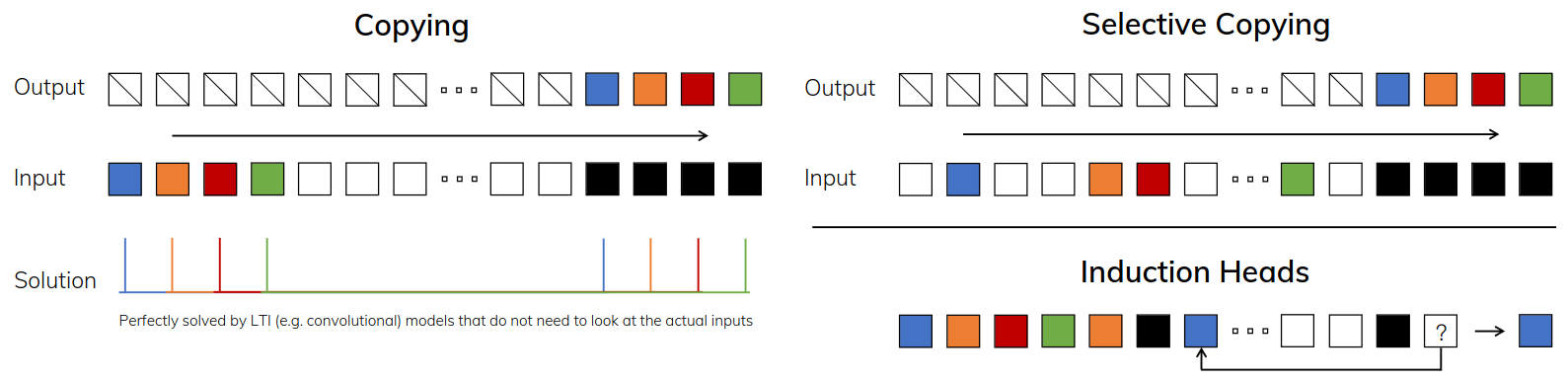
- Left: Copying task
- Constant spacing between input and output elements
- Easily solved by time-invariant models such as linear recurrences and global convolutions
- Right Top: Selective Copying task
- Random spacing in between inputs
- Requires time-varying models that can selectively remember or ignore inputs depending on their content
- Right Bottom: The Induction Heads task
- Associative recall: requires retrieving an answer based on context
- A key ability for LLMs
Problems of LTI models
- Recurrent view
- LTI model implies constant dynamics / Fixed $(\bar{A},\bar{B})$
- LTI model cannot
- Select the correct information from their context
- Affect the hidden state passed along the sequence an in input-dependent way
- Convolutional view
- Global convolutions can solve the vanilla Copying task because it only requires time-awareness
- Global convolutions cannot solve Selective Copying task because of lack of content-awareness
- The spacing between inputs-to-outputs is varying and cannot be modeled by static convolution kernels
The Tradeoff
- Efficient models: must have a small state
- Effective models: must have a state that contains all necessary information from the context
The authors propose that a fundamental principle for building sequence models is selectivity
- Allow model to focus on or filter out inputs into a sequential state
- Allow model to controls how information propagates or interacts along the sequence dimension
Selection Mechanism
- Key observation: model parameters should be input-dependent
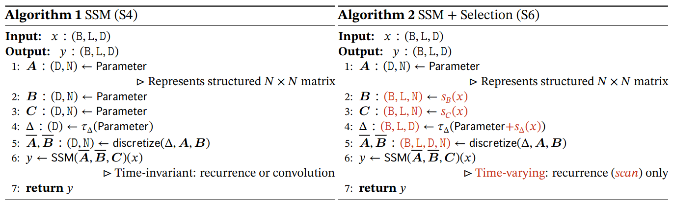
Main difference between S4 and S6
- In S6, parameters $\Delta, B, C$ are functions of the input $x$
- Parameters now have a length dimension $L$
- The model has changed from time-invariant to time-varying
- Recurrency cannot be converted in convolutions
- S6 projections
- $\text{Linear}_d$: parameterized projection to dimension $d$
- $s_B(x) = \text{Linear}_N(x)$
- $s_C(x) = \text{Linear}_N(x)$
- $s_\Delta(x) = \text{Broadcast}_D(\text{Linear}_1(x))$
- $\tau_\Delta = \text{softplus}$
- Choice of $s_\Delta$ and $\tau_\Delta$ is due to a connection to RNN gating mechanisms
Efficient Implementation of Selective SSMs
Motivation
- Input $x$ and output $y$ are of shape $(B,L,D)$
- However, running SSM in recurrent mode requires materializing the latent state $h$ with shape $(B,L,D,N)$
- Efficient convolution mode
- This mode could bypass the state computation
- Materializes a convolution kernel $\bar{K} = (…)$ of only $(B,L,D)$
Selective Scan: Hardware-Aware State Expansion
Address computation problem of non-LTI model with three classical techniques:
- Kernel fusion
- Parallel scan
- Recomputation
Main observations
- Computation Cost
- Recurrent: $O(BLDN)$, with a lower constant factor
- Convolutional: $O(BLD\log(L))$
- For long sequences and small state dimension $N$, the recurrent mode induce fewer FLOPs
- Two challenges of Recurrent mode
- Sequential nature of recurrence
- Large memory usage (can be addressed by not materialize the full state $h$)
Main idea
- Materialize the state $h$ only in more efficient levels of the memory hierarchy
- Most operations (except MatMul) are memory bounded, includes scan operation
- Use kernel fusion to reduce memory IOs, leading to a significant speedup
Procedure
- Instead of preparing the scan input $(\bar{A},\bar{B})$ of size $(B,L,D,N)$ in GPU HBM
- Load the SSM parameters $(\Delta, A, B, C)$ directly from slow HBM to fast SRAM
- Perform the discretization and recurrence in SRAM
- Then write the final outputs of size $(B,L,D)$ back to HBM
Avoid the sequential recurrence
- Despite not being linear, the SSM can still be parallelized with a work-efficient parallel scan algorithm
Avoid saving the intermediate states
- Intermediate states are required for backpropagation
- Solution: recomputation
- Intermediate states are not stored but recomputed in the backward pass
- Recomputation are performed when the inputs are loaded from HBM to SRAM
- Reduce the memory requirements
- Details of the fused kernel and recomputation are in Appendix D
A Simplified SSM Architecture
Selective SSMs are standalone sequence transformations that can be incorporated into neural networks
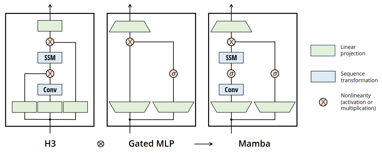
Architecture
- Expanding the model dimension $D$ by a controllable expansion factor $E$
- For each block
- Most of the parameters ($3ED^2$) are in the linear projections
- $2ED^2$ for input projections
- $ED^2$ for output projection
- SSM parameters are much smaller in comparison
- Projections for $\Delta, B, C$
- Matrix $A$
- $\sigma$: SiLU / Swish activation
- Most of the parameters ($3ED^2$) are in the linear projections
- Composition of Mamba block
- Interleave with standard normalization and residual connections
- Optional LayerNorm
Properties of Selection Mechanisms
Selection mechanism is a general technique
- Can be applied to RNNs or CNNs
- Can be applied to different parameters
- Can adopt different transformations $s(x)$
Connection to Gating Mechanisms
- RNN’s Gating mechanism is a special case of selection mechanism
- $\Delta$ in SSMs can be seen to play a generalized role of the RNN gating mechanism
Theorem 1
When $N=1, A=-1, B=1, s_\Delta=\text{Linear}(x), \tau_\Delta=\text{softplus}$, then the selective SSM recurrence (Algorithm 2) takes the form:
\[\begin{align} g_t &= \sigma(\text{Linear}(x_t)) \\ h_t &= (1-g_t)h_{t-1} + g_t x_t \end{align}\]Note that if a given input $x_t$ should be completely ignored (as necessary in the synthetic tasks), all $D$ channels should ignore it, and so we project the input down to 1 dimension before repeating/broadcasting with $\Delta$.
Interpretation of Selection Mechanisms
Variable Spacing
- Selectivity allows filtering out irrelevant noise tokens
- The Selective Copying task is an extreme example
- However, this type of filtering is ubiquitously in common data modalities, particularly for discrete data
- For example, the presence of language fillers such as “um”
Filtering Context
- Long context
- In theory, More context should lead to strictly better performance
- In practice, many sequence models do not improve with longer context
- Possible that sequence models (e.g., global convolutions / LTI) cannot effectively ignore irrelevant context
- In comparison, selective models can reset their state to remove extraneous history
Boundary Resetting
- For multiple independent sequences are stitched together
- Transformers can keep independent sequences separated by attention mask
- LTI models will blend information between sequences
- Selective SSMs can reset their state at sequence boundaries
Interpretation of $\Delta$
- View 1: $\Delta$ controls how much to focus or ignore the current input $x_t$
- Large $\Delta$: resets the state $h$ and focuses on the current input $x$
- Small $\Delta$: persists the state and ignores the current input
- View 2: a continuous system discretized by a timestep $\Delta$
- Large $\Delta \to \infty$: the system focusing on the current input for longer (select $x$, forget $h$)
- Small $\Delta \to 0$: transient input that is ignored
Interpretation of $A$
- $A$ affects the model only through its interaction with $\Delta$ via $\bar{A} = \exp(\Delta A)$
- In comparison, selectivity from $\Delta$ affect both $\bar{A}$ and $\bar{B}$
Interpretation of $B$ and $C$
- Modifying $B$ and $C$ to be selective allows finer-grained control over
- Whether to let an input $x_t$ into the state $h_t$
- Whether to let an state $h_t$ into the output $y_t$
- Allow the model to modulate the recurrent dynamics based on
- Content (input $x$)
- Context (hidden states $h$)
Additional Model Details
Real vs. Complex
- Most prior SSMs use complex numbers in state $h$, which is necessary for strong performance on many tasks
- Ref: [Efficiently Modeling Long Sequences with Structured State Spaces]
- Empirically observed that completely real-valued SSMs seem to work fine, and possibly even better, in some settings
- Ref: [Mega: Moving Average Equipped Gated Attention, ICLR 2023]
- Mamba: default to real values, work well for all but one of our tasks
- Hypothesize
- Complex-real tradeoff is related to the continuous-discrete spectrum in data modalities
- Complex numbers: helpful for continuous modalities (e.g. audio, video)
- Real numbers: helpful for discrete modalities (e.g. text, DNA)
Initialization
- Most prior SSMs requires special initializations, particularly in the complex-valued case
- Mamba’s default initialization of $A$
- Complex: S4D-Lin ( n-th diagonal: $-1∕2 + ni$ )
- Real: S4D-Real ( n-th diagonal: $-(n+1)$ )
- Based on HiPPO theory
- Ref: [On the Parameterization and Initialization of Diagonal State Space Models, NIPS 2022]
- Many initializations should work fine, particularly in the large-data and real-valued SSM regimes
Parameterization of $\Delta$
Selective adjustment $\Delta$:
\[s_\Delta (x) = \text{Broadcast}_D(\text{Linear}_1 (x))\]Notes
- Linear Projection can be generalized from dimension 1 to a larger dimension $R$ (still $R < D$)
- Broadcasting operation can be viewed as another Linear projection, initialized to a specific pattern of 1 and 0
- If Broadcasting projection is trainable
- $s_\Delta (x) = \text{Linear}_D (\text{Linear}_R (x))$
- This can be viewed as a low-rank projection
- $\Delta$ parameter is initialized to $\tau_\Delta^{-1}(\text{Uniform}([0.001, 0.1]))$
- Ref: [How to Train Your HIPPO: State Space Models with Generalized Basis Projections, ICLR 2023]
Sometimes selective SSMs is abbreviated as S6 models, because they are S4 models with a selection mechanism and computed with a scan.
Experiments
Synthetic Tasks
Selective Copying
- LTI SSMs can easily solve Copying task by only keeping track of time instead of reasoning about the data
- Ref: [CKConv: Continuous Kernel Convolution For Sequential Data, 2021]
- Previous work
- Architecture gating (multiplicative interactions) can endow models with “data-dependence”
- However, such gating
- Does not interact along the sequence axis
- Cannot affect the spacing between tokens
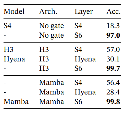
Gated architectures such as H3 and Mamba only partially improve performance, while the selection mechanism (modifying S4 to S6) easily solves this task.
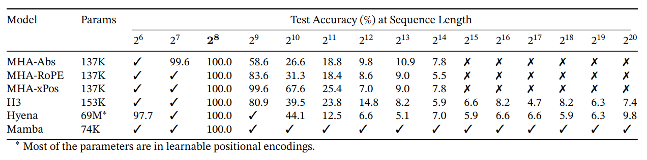
Induction Heads
- Surprisingly predictive of the in-context learning ability of LLMs
- Requires models to perform associative recall and copy
- If the model has seen a bigram such as “Harry Potter” in the sequence
- Then the next time “Harry” appears, the model should predict “Potter” by copying from history
- Dataset
- Training
- Vocab size: 16
- Sequence length: 256
- Testing
- Sequence length: 64 - 1,048,576
- Training
- Model
- 2 layer Models
- Model types: 8-head attention, SSM variants
- $D = 64$ or $D = 128$
Mamba is trained on sequence length $2^8 = 256$, but generalizes perfectly to million-length sequences, or 4000x longer than it saw during training, while no other method goes beyond 2x.
Language Modeling
- Dataset: the Pile
Scaling Laws
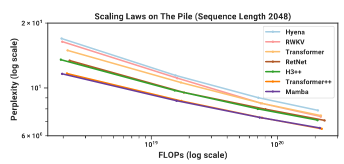
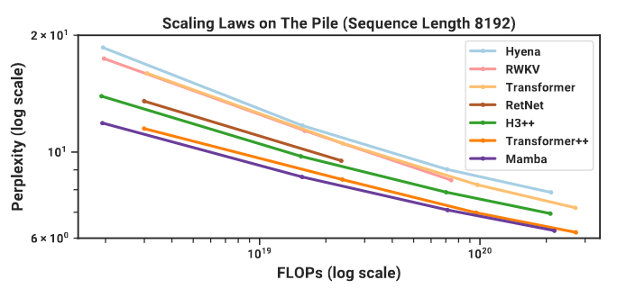
Models of size from 125M to 1.3B parameters. Mamba scales better than all other attention-free models and is the first to match the performance of a very strong “Transformer++” (PaLM and LLaMa architectures: rotary embedding, SwiGLU MLP, RMSNorm instead of LayerNorm, no linear bias, and higher learning rates).
Downstream Evaluations
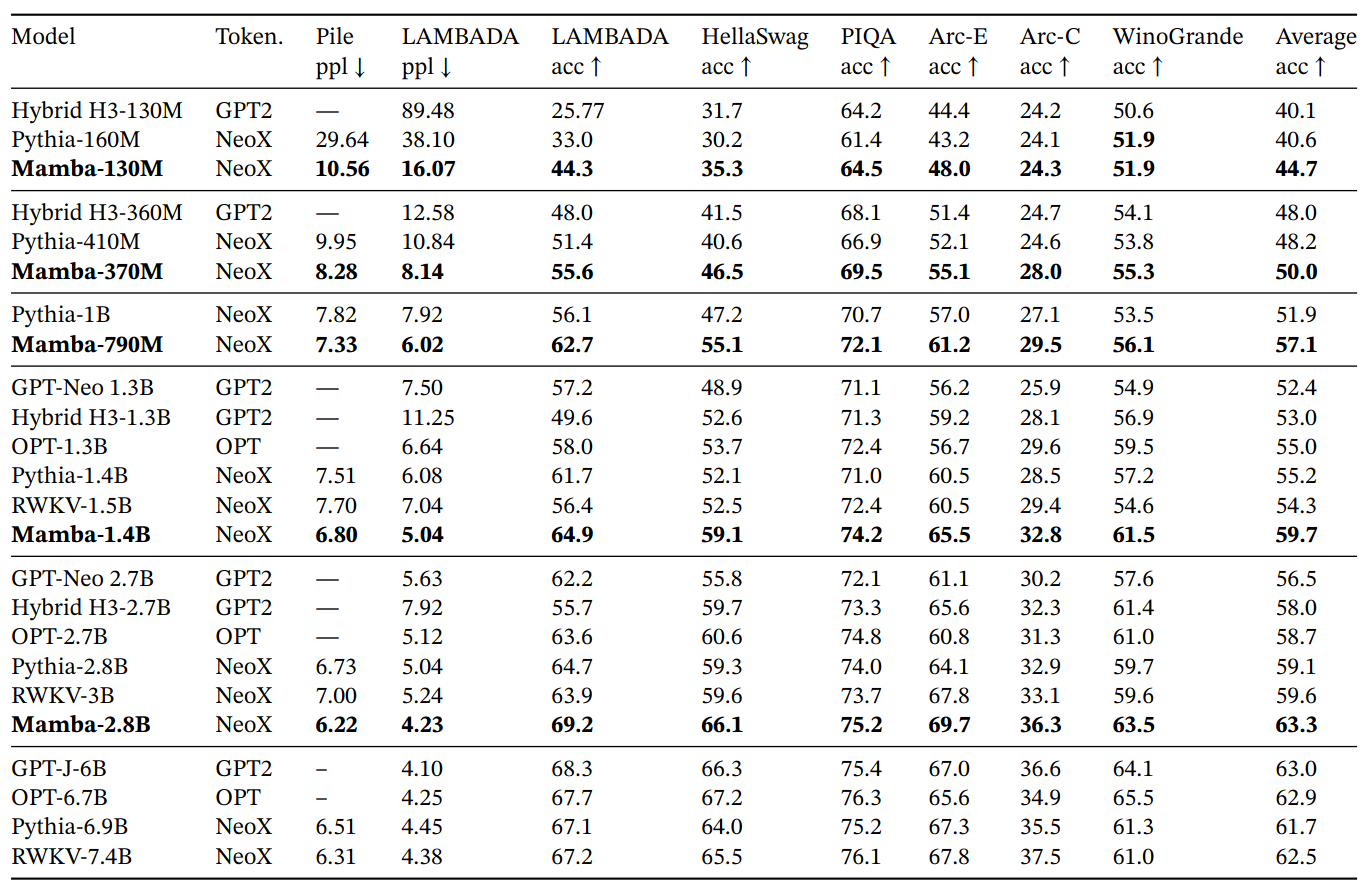
Open source LMs with various tokenizers, trained for up to 300B tokens. Pile refers to the validation split, comparing only against models trained on the same dataset and tokenizer (GPT-NeoX-20B). For each model size, Mamba is best-in-class on every single evaluation result, and generally matches baselines at twice the model size.
DNA Modeling
- Pre-training: standard causal language modeling (next token prediction)
- Dataset: HG38, single human genome with about 4.5 billion tokens (DNA base pairs) in the training split (follow HyenaDNA)
Scaling: Model Size
- Sequence length: 1024
- Global batch size: 1024
- ~1M tokens per batch
- Model trained for 10K gradient steps for a total of 10B tokens
Scaling: Context Length
- Model size: 6 layers by width 128 (~1.3M-1.4M parameters)
- Pretrained on sequence length 1024-1,048,576
- Trained for 20K gradient steps for a total of ~330B tokens
- Sequence length warmup
- Ref: [HyenaDNA: Long-range Genomic Sequence Modeling at Single Nucleotide Resolution, NIPS 2023]
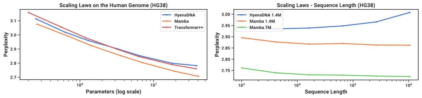
Left: Model Size Scaling, Mamba can match the Transformer++ and HyenaDNA models with roughly 3x to 4x fewer parameters.
Right: Context Length Scaling, Mamba pretraining perplexity improves up to sequences of length 1M.
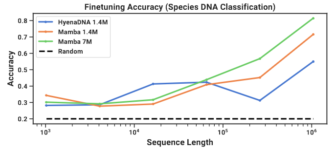
Synthetic Species Classification
- Downstream task: classifying between 5 different species by randomly sampling a contiguous segment of their DNA
- Classifying between the five great apes species {human, chimpanzee, gorilla, orangutan, bonobo}, which are known to share 99% of their DNA
- Fine-tuning on sequences of length 1024-1,048,576 using pretrained models of the same context length
Audio Modeling and Generation
- Benchmark: SaShiMi architecture
- U-Net backbone
- Alternating S4 and MLP blocks in each stage
- Mamba: replacing the S4+MLP blocks with Mamba blocks
Long-Context Autoregressive Pretraining
- Pretraining
- YouTubeMix, piano music dataset / 4 hours of solo piano 16000 Hz
- Sequence lengths: 8192 - $10^6$
- Use complex parameterization, instead of real parameterization
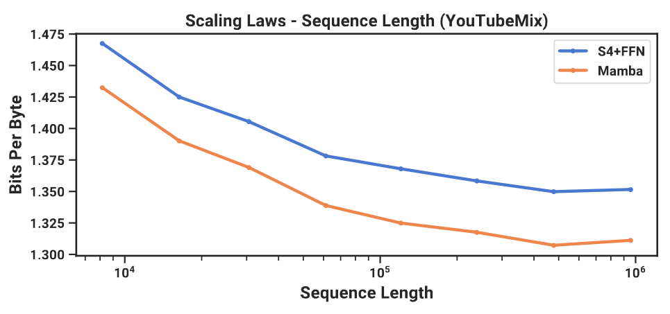
Mamba outperforms SOTA Sashimi in autoregressive audio modeling.
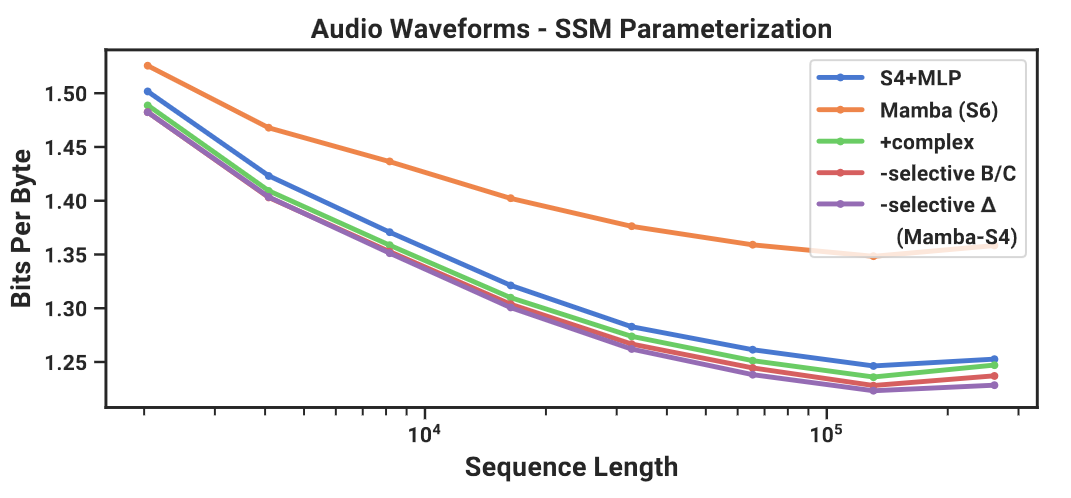
- Change from S4 to S6 (add the selection mechanism) is not always beneficial
- Audio is uniformly sampled and very smooth, and therefore benefits from continuous linear time-invariant (LTI) methods
- Best model: S4 layer inside the Mamba block, Mamba-S4 (complex, remove selective $B,C$ and $\Delta$)
Speed and Memory Benchmarks
- Efficient SSM scan
- Faster than FlashAttention-2 beyond sequence length 2K
- Up to 20-40x faster than a standard scan implementation in PyTorch
- Mamba
- 4-5x higher inference throughput than a Transformer of similar size
- Removing KV cache allow Mamba use much higher batch sizes
Model Ablations
Setup: Language modeling with 350M-models at Chinchilla token counts
SSM Architecture
- All non-selective/LTI SSMs have similar performance
- Complex S4 => real S4 does cause performance degradation (real-valued SSMs may be preferred considering hardware efficiency)
- Replacing any non-selective layer (S4/Hyena) with selective layer (S6) significantly improves performance
- Mamba and H3 performs similarly
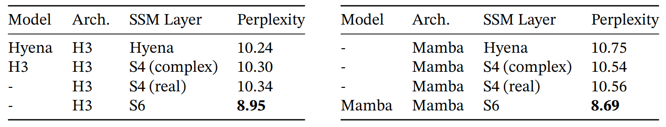
S4 (real): S4D-Real; S4 (complex): S4D-Lin.
Selective Layer Parameterization
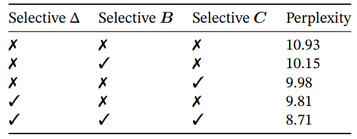
Ablations: Selective parameters; $\Delta$ is the most important parameter; Multiple selective parameters create synergy.
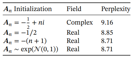
Ablations: Parameterization of A. Real-valued diagonal initializations performs better than complex-valued parameterizations. Random initializations also work well.
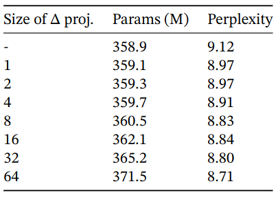
Ablation: dimension of the $\Delta$. State size fixed to 16. Projecting input even to 1-dim $\Delta$ resulting in large performance gain. Increasing $\Delta$ dimension provides further improvements at the modest cost in parameters.
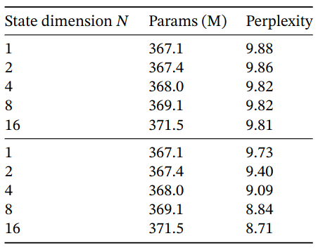
Ablation: dimension of the $B,C$. $\Delta$ projection fixed to 64. Top: constant $B,C$; Bottom: selective $B,C$. SSM state dimension $N$ can be viewed as an expansion factor on the dimension of the recurrent state. For selective $B,C$, increasing $N$ significantly boost LM performance at a negligible cost in parameters/FLOPs.
Discussion
No Free Lunch: Continuous-Discrete Spectrum
- SSMs were originally defined as discretizations of continuous systems
- SSMs have had a strong inductive bias toward continuous-time data modalities
- The selection mechanism
- Overcomes SSMs weaknesses on discrete modalities (text and DNA)
- Impede SSMs performance on data that LTI SSMs excel on (audio waveforms)