S5 & Parallel Scan
This post is mainly based on
Parallel Scan
Scan Operation
Given a binary associative operator $\bullet$ and a sequence of $L$ elements $[a_1, a_2, …, a_L]$, the scan operation (or all-prefix-sum operation) returns the sequence:
\[\left[ a_1, \; (a_1 \bullet a_2), \; \ldots, \; (a_1 \bullet a_2 \bullet \ldots \bullet a_L) \right]\]Parallel Scan Operation
The parallelization of scan operations has been well studied in
- [Prefix sums and their applications, 1990]
- [Parallel computing using the prefix problem, 1994]
Many standard scientific computing libraries contain efficient implementations.
Naive Parallel Scan
A naive algorithm take advantage of the parallel processing and have time complexity $O(\log_2 n)$.
However, this algorithm is not compute-efficient: while a sequential sum requires $n$ operations, the naive algorithm requires $O(n \log_2 n)$ operations. At level $d=1$, the algorithm assumes that there is $n-1$ parallel processes can be called, which is not realistic for large array.
Observe that there are a lot of redundant operations. For example, to compute $\sum (x_0, …, x_4)$. The naive algorithm performs 3 operations
- $x_3 + x_4$
- $(x_1 + x_2) + (x_3 + x_4)$
- $x_0 + (x_1 + x_2) + (x_3 + x_4)$
A more efficient way is to wait until $\sum (x_0, …, x_3)$ is computed, the perform a single operation $\sum (x_0, …, x_3) + x_4$. To achieve this, we need to design an algorithm to determine which sum to execute first and which sum to hold.
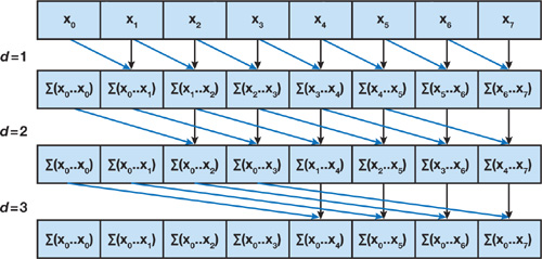
Compute-Efficient Parallel Scan
To determine which the optimal sequence of operations, we build a balanced binary tree:

In the Up-Sweep (Reduce) Phase, we perform pairwise operations at each level to compute partial sum for all even index elements and hold the intermediate result.
The root node $\sum(x_0, …, x_7)$ is therefore computed, since it holds the sum of all nodes in the array.
In the Down-Sweep Phase, we perform a sequence of shuffle and addition operations, where:
- At level $d=0$, initialize the root node to 0
- At each subsequent level $d$
- Identify $2^d$ nodes at this level
- For each node, assume they hold intermediate values:
- Node: $x_p$
- Left child: $x_l$
- Right child: $x_r$
- Perform the following operations
- Left child = $x_p$
- Right child = $x_p + x_l$
The resulting sequence will be the all-prefix-sum excluding the last element, which was computed in the Up-Sweep Phase.
This algorithm
- Has time complexity $2 \log_2 n$, if we can compute $n/2$ additions in parallel
- Requires $2(n - 1)$ additions, $n - 1$ swaps
Note that
- In this example, we use addition $+$, which is an associative operator
- Parallel scan works on any associative operator
- An associative operator is not necessarily commutative, therefore the right child must be computed in $x_p + x_l$, not $x_l + x_p$
Parallel Scan on SSM
Parallel Scan requires binary associative operator. Therefore, we need to propose an associative operator for SSM updates.
Let $\bullet$ be:
\[q_i \bullet q_j := ( q_{j,a} \odot q_{i,a}, \quad q_{j,a} \otimes q_{i,b} + q_{j,b} )\]where
- $\odot$: matrix-matrix multiplication
- $\otimes$: matrix-vector multiplication
- $+$: element-wise addition
It can be shown that $\bullet$ operator is associative.
To show what this $\bullet$ operator is equivalent to a state update in SSM, let’s consider the following example.
An Example
Consider a linear state update $x_k = \bar{A} x_{k-1} + \bar{B} u_k$, $u_{1:4}$ and $x_0=0$. We have:
\[\begin{align} x_1 &= \bar{B} u_1\\ x_2 &= \bar{A}\bar{B} u_1 + \bar{B} u_2\\ x_3 &= \bar{A}^2\bar{B} u_1 + \bar{A}\bar{B} u_2 + \bar{B} u_3\\ x_4 &= \bar{A}^3\bar{B} u_1 + \bar{A}^2\bar{B} u_2 + \bar{A}\bar{B} u_3 + \bar{B} u_4\\ \end{align}\]Sequential Compute
To show why $\bullet$ operator is equivalent to a state update in SSM, define $c_{1:L}$, where each element $c_k$ is the tuple:
\[c_k = (c_{k,a}, \: c_{k, b}) := (\bar{A}, \: \bar{B} u_k )\]Note that $c_{1:L}$ can be easily initialize prior to parallel scan.
To compute the recurrence sequentially, initialize $c_{1:4}$ and $s_0$ as:
\[\begin{align} c_{1:4} &:= ( (\bar{A}, \: \bar{B} u_1 ), (\bar{A}, \: \bar{B} u_2 ), (\bar{A}, \: \bar{B} u_3 ), (\bar{A}, \: \bar{B} u_4 ) ) \\ s_0 &:= (I, 0) \end{align}\]where $I$ is identity matrix.
Then we have:
\[\begin{align} s_1 &= s_0 \bullet c_1 = (I, 0) \bullet (\bar{A}, \bar{B} u_1) = (\bar{A}, \bar{B} u_1) \\ s_2 &= s_1 \bullet c_2 = (\bar{A}^2, \bar{A}\bar{B} u_1 + \bar{B} u_2)\\ s_3 &= s_2 \bullet c_3 = (\bar{A}^3, \bar{A}^2\bar{B} u_1 + \bar{A}\bar{B} u_2 + \bar{B} u_3)\\ s_4 &= s_3 \bullet c_4 = (\bar{A}^4, \bar{A}^3\bar{B} u_1 + \bar{A}^2\bar{B} u_2 + \bar{A}\bar{B} u_3 + \bar{B} u_4)\\ \end{align}\]Note that the second element in the tuple $s_i$ is the Linear SSM state update result.
Parallel Scan
Let’s compute this scan operation using parallel scan.
First execute the Up-Sweep Phase:
d = 1:
\[\begin{align} r_{2, d=1} &:= c_1 \bullet c_2 \\ r_{4, d=1} &:= c_3 \bullet c_4 \\ \end{align}\]d = 2:
\[r_{4, d=2} := r_{2, d=1} \bullet r_{4, d=1} = (c_1 \bullet c_2) \bullet (c_3 \bullet c_4)\]This is the final element of the parallel scan.
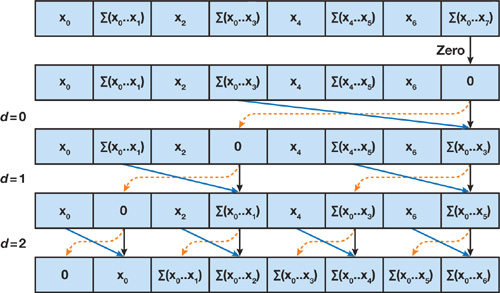
Then execute the Down-Sweep Phase:
Set $r_{4, d=0} = (I, 0)$
d = 1:
For node $r_{4, d=0} = (I, 0)$,
- Left child $r_{2, d=1} = (I, 0)$
- Right child $r_{4, d=1} = (I, 0) \bullet r_{2, d=1} = c_1 \bullet c_2$
d = 2:
For node $r_{4, d=1} = c_1 \bullet c_2$,
- Left child $r_{3, d=1} = r_{2, d=1} = c_1 \bullet c_2$
- Right child $r_{4, d=1} = r_{2, d=1} \bullet c_3 = (c_1 \bullet c_2) \bullet c_3$
For node $r_{2, d=1} = (I, 0)$,
- Left child $r_{1, d=1} = (I, 0)$
- Right child $r_{2, d=1} = (I, 0) \bullet c_1 = c_1$
Excluding the first element $(I, 0)$, we end up with the remaining $n-1$ elements of the parallel scan:
\[[c_1, c_1 \bullet c_2, c_1 \bullet c_2 \bullet c_3]\]S5
- S4 vs S5
- S4 layer: many independent SISO (single input single output) SSMs
- S5 layer: one MIMO (multi input multi output) SSM
- S5
- $A$ is diagonalized, similar to S4D
- Recurrent computation only, no Convolution
- Parallel scan can match computational efficiency of S4
- Can handle time-varying SSMs and irregularly sampled observations
- Results
- SOTA on several long-range sequence modeling tasks
Background
Linear State Space Model
Continuous-time linear SSMs:
\[\begin{align} x'(t) &= Ax(t) + Bu(t)\\ y(t) &= Cx(t) + Du(t) \end{align}\]Given a constant step size $\Delta$, the continuous SSM can be discretized:
\[\begin{align} x_k &= \bar{A}x_{k-1} + \bar{B}u_k\\ y_k &= \bar{C}x_k + \bar{D}u_k \end{align}\]with Euler, bilinear or zero-order hold (ZOH) methods.
Linear SSM with Parallel Scan
A length $L$ linear recurrence of a discretized SSM can be computed by the scan operation.
Complexity
Given $L$ processors, the linear recurrence of the discretized SSM above can be computed in a parallel time of $O(T_\odot \log L)$, where $T_\odot$ is the cost of matrix-matrix multiplication.
For diagonal matrix $\bar{A} \in \mathbb{R}^{P \times P}$, the time cost of $T_\odot$ is $O(P\log L)$ and space cost is $O(PL)$.
S4 Layer
Given a sequence of length $L$ and channel $H$, the S4 layer defines a nonlinear sequence-to-sequence mapping:
- From an input sequence: $u_{1:L} \in \mathbb{R}^{L \times H}$
- To an output sequence: $u’_{1:L} \in \mathbb{R}^{L \times H}$
An S4 layer contains $H$ independent single-input, single-output (SISO) SSMs
- Each SSM
- Has $N$-dimensional states
- Leverages the HiPPO framework for online function approximation
- The HiPPO-LegS matrix can be reduce to a normal plus low-rank (NPLR/DPLR) form
- Each SSM applied to a single dimension of the input sequence
- This results in an independent linear transformation from each input channel to each preactivation channel
- Then, a nonlinear activation function is applied to each preactivation channel
- Finally, a position-wise linear mixing layer is applied to combine the activation
- This results in the output sequence $u’_{1:L}$
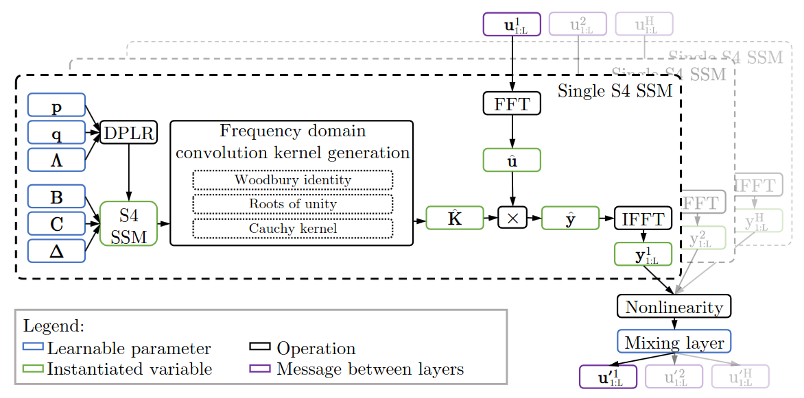
S4 layer
S4 Learnable parameters
- $H$ independent SSM
- Input matrix: $B^{(h)} \in \mathbb{C}^{N \times 1}$
- DPLR parameterized transition matrix $A^{(h)} \in \mathbb{C}^{N \times N}$
- Output matrix $C^{(h)} \in \mathbb{C}^{1 \times N}$
- Timescale parameter $\Delta(h) \in \mathbb{R}_+$
- Mixing layer: $O(H^2)$ parameters
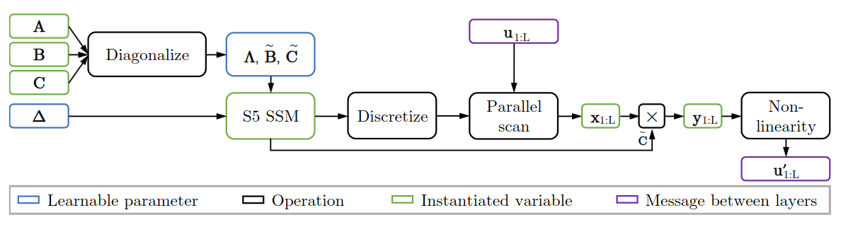
S5 Layer
The S5 layer replaces $H$ independent SISO SSMs with a multi-input, multi-output (MIMO) SSM.
S5 layer
S5 Parameterization
Given $A$ is diagonalizable: $A = V \Lambda V^{-1}$, where $\Lambda \in \mathbb{C}^{P \times P}$, then the continuous-time latent dynamics is also diagonalizable:
\[\frac{dV^{-1}x(t)}{dt} = \Lambda V^{-1}x(t) + V^{-1}Bu(t)\]Let $\tilde{x}(t) = V^{-1}x(t)$, $\tilde{B} = V^{-1}B$, and $\tilde{C} = CV$, then the reparameterized system is:
\[\begin{align} \frac{d\tilde{x}(t)}{dt} &= \Lambda \tilde{x}(t) + \tilde{B}u(t)\\ y(t) &= \tilde{C}\tilde{x}(t) + Du(t) \end{align}\]This is a linear SSM with a diagonal state matrix. This diagonalized system can be discretized with a timescale parameter $\Delta \in \mathbb{R}_+$ using the ZOH method to give another diagonalized system with parameters
\[\begin{align} \bar{\Lambda} &= e^{\Lambda \Delta} \\ \bar{B} &= \Lambda^{-1}(\Lambda - I)\tilde{B} \\ \bar{C} &= \tilde{C} \\ \bar{D} &= D \end{align}\]In practice,
- $\Delta \in \mathbb{R}^P$: vector of learnable timescale parameters
- $D$: restrict to be diagonal
S5 Learnable parameters
- $\tilde{B} \in \mathbb{C}^{P \times H}$
- $\tilde{C} \in \mathbb{C}^{H \times P}$
- $\text{diag}(D) \in \mathbb{R}^H$
- $\text{diag}(\Lambda) \in \mathbb{C}^P$
- $\Delta \in \mathbb{R}^P$
S5 Layer
- 1 MIMO SSM
- Latent state size $P$
- Input and output dimension $H$
- Map input $u_{1:L} \in \mathbb{R}^{L \times H}$ to output $y_{1:L} \in \mathbb{R}^{L \times H}$
- Then, a nonlinear activation function is applied to produce $u’_{1:L} \in \mathbb{R}^{L \times H}$
- No mixing layer required, since these features are already mixed
- S5 vs S4: S4’s $H$ independent SSM can be viewed as a block-diagonal system
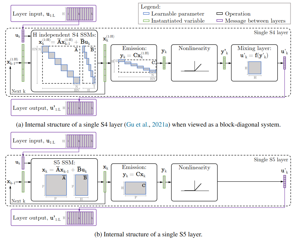
Internal structure of a discretized S4 layer vs S5 layer. S4 layer: single block-diagonal SSM with a latent state of size $HN$, followed by a nonlinearity and mixing layer to mix the independent features; S5 layer: dense linear SSM with latent size $P \ll HN$.
Initialization
Initializing S5 with HiPPO-like matrices may also work well in the MIMO setting.
The empirical results show that diagonalizing the HiPPO-N matrix leads to good performance.
[TBD: Appendix E]
Irregularly Spaced Time Series
Parallel scans and the continuous-time parameterization also allow for efficient handling of irregularly sampled time series. This can be achieved by supplying a different $\bar{A}_k$ matrix at each step.
In contrast, the convolution of the S4 layer requires a time invariant system and regularly spaced observations.
Relationship Between S4 and S5
[TBD]
Experiments
Long Range Arena
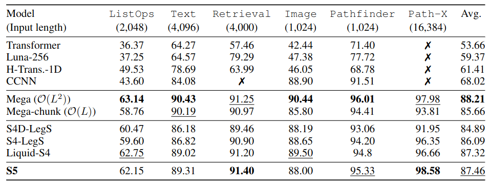
LRA benchmark. The best Mega model retains the transformer’s $O(L^2)$ complexity.
Speech Classification
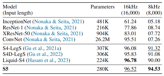
Test accuracy on 35-way Speech Commands classification task. Training examples are one-second 16kHz audio waveforms.
Irregularly Spaced Time Series
Pendulum regression requires model to handle observations received at irregular intervals.
Input
- A sequence of $L=50$ images,
- Each 24 $\times$ 24 pixels in size
- Each has been corrupted with a correlated noise process
- Image sampled at irregular intervals from a continuous trajectory of duration $T = 100$
- The velocity is unobserved
Target
- Sine and cosine of the angle of the pendulum
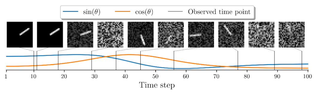
Illustration of the pendulum regression example.
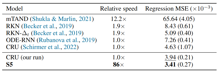
Regression MSE $\times 10^{−3}$ (mean +/- std) and relative application speed on the pendulum regression task on a held-out test set. Results for CRU (our run) and S5 are across twenty seeds.