S4D: Diagonal State Space Models
This post is mainly based on
- Stable DPLR: It’s Raw! Audio Generation with State-Space Models
- DSS: Diagonal State Spaces are as Effective as Structured State Spaces, NIPS 2022
- S4D: On the Parameterization and Initialization of Diagonal State Space Models, NIPS 2022
Relationship between 4 papers
- S4 / DPLR
- $A = V\Lambda V^\top + PQ^\top$
- Parameterize $A$ via a diagonal plus low rank (DPLR) structure
- Stable DPLR
- $A = V\Lambda V^\top - PP^\top$
- HiPPO matrices admit this restrictive parameterization
- This parameterization can be better controlled to be numerically stable during autoregressive generation
- DSS
- $A \approx V\Lambda V^\top$
- Theoretically, HiPPO-LegS matrix cannot be stably transformed into diagonal form (S4 paper’s Lemma 3.2)
- Empirical observation: removing the low rank portion from DPLR results in a model performs comparably to the original S4
- Requires zero-order hold (ZOH) Discretization
- S4D
- Systematically analyze the DSS
- Mathematically show why diagonalization of $A$ works
- Admits both Bilinear and ZOH Discretization
Stable DPLR
- Improve the parameterization of S4
- Identify that S4 can be unstable during autoregressive generation
- Provide a simple improvement to its parameterization, ensuring stability when switching into recurrent mode
Background
What is spectrum?
- The spectrum of a matrix is the set of eigenvalues of that matrix
- If all eigenvalues of $A$ have absolute values less than 1, the system is stable
- If any eigenvalue has an absolute value greater than 1, the system is unstable
Stable DPLR
Definition A Hurwitz matrix A is one where every eigenvalue has negative real part
Hurwitz matrices are also called stable matrices, because they imply that the SSM is asymptotically stable.
Example: Consider a discrete time SSMs:
\[\begin{align} h_k &= \bar{A}h_{k-1} + \bar{B}x_k \\ y_k &= Ch_k + Dx_k \end{align}\]Unrolling $h_k$ in the RNN mode involves powering up A repeatedly, which is stable if and only if all eigenvalues of $A$ lie inside or on the unit disk.
Discretized State Matrix
\[\bar{A} = (I - \Delta/2 \cdot A)^{-1} (I + \Delta/2 \cdot A)\]This transformation maps the complex left half plane (i.e. negative real part) to the complex unit disk
Therefore, if $A$ is Hurwitz matrix, $\bar{A}$ is unitary, hence the implied SSMs is stable.
Proposition A matrix $A = \Lambda - PP^\top$ is Hurwitz if all entries of $\Lambda$ have negative real part.
This implies that under Stable DPLR, controlling the spectrum of the learned $A$ can be achieved by controlling the the diagonal portion $\Lambda$, which is far easier than controlling a general DPLR matrix.
Proposition All three HiPPO matrices from are unitarily equivalent to a matrix of the form $A = \Lambda - PP^\top$ for diagonal $\Lambda$ and $p \in \mathbb{R}^{N \times r}$ for $r = 1$ or $r = 2$. Furthermore, all entries of $\Lambda$ have
- Real part $0$ (for HiPPO-LegT and HiPPO-LagT)
- Real part $-1/2$ (for HiPPO-LegS)
This implies all HiPPO matrices are Hurwitz.
Empirically, the authors found that S4 matrices generally became non-Hurwitz after training.
Note
- The stability issue only arises when using S4 during autoregressive generation
- S4’s convolutional mode during training does not involve powering up A and thus does not require a Hurwitz matrix
Diagonal State Spaces (DSS)
- S4 parameterize the state update matrix $A$ via a diagonal plus low rank (DPLR) structure
- DSS removes the low rank correction from DPLR
- Findings
- DSS can match the performance of S4
- DSS is competitive to S4 on Long Range Arena and speech classification on SC
- Since $A$ is fully diagonal, DSS conceptually simpler and straightforward to implement
We skip details of this paper since S4D is more comprehensive and easier to follow.
Diagonal State Space Models (S4D)
- Systematically understand how to parameterize and initialize DSS models
- Initialization is critical for performance
- Mathematically show that the diagonal restriction of S4’s matrix surprisingly recovers the same kernel in the limit of infinite state dimension
- S4D
- Diagonal version of S4 whose kernel computation requires just 2 lines of code
- Competitive to S4 in almost all settings (image, audio, and medical time-series)
Background
Continuous State Spaces Models
The SSMs implied by S4 can be represented either as a linear ODE:
\[\begin{align} x'(t) &= Ax(t) + Bu(t)\\ y(t) &= Cx(t) \end{align}\]or a convolution
\[\begin{align} K(t) &= Ce^{tA}B\\ y(t) &= (K * u)(t) \end{align}\]Why the LTI Form and the Convolution Form are equivalent?
Consider the homogeneous equation, where $u(t) = 0$. This represent how the state involves without external input $u(t)$. We have $x’(t) = Ax(t)$. Consider ODE $x’(t) = ax(t)$ with a scalar $a$, which is a separable equation:
\[\begin{align} \frac{1}{x} dx &= a dt \\ \int \frac{1}{x} dx &= \int a dt \\ \ln |x| &= at + \alpha \\ x &= \alpha' e^{at} \end{align}\]This technique is generalizable to matrix $A$ and the $e^{At}$ term in the convolution kernel $K(t) = Ce^{tA}B$ comes from solving the homogeneous equation.
Next, we need to take $u(t)$ into consideration. Below is Differential Equation with impulse input:
\[x'(t) = Ax(t) + B\delta(t)\]where $\delta(t)$ is a Dirac delta function representing an impulse input at time $t=0$.
Applying Laplace Transform to solve the differential equation with the impulse input:
- Linearity: The Laplace transform of a sum is the sum of the Laplace transforms.
- Differentiation: If \(L \{ x(t) \}=X(s)\), then \(L \{x'(t)\} = sX(s) - x(0)\).
- Delta Function: The Laplace transform of the Dirac delta function is 1, $L{\delta(t)}=1$
Assume $x(0) = 0$
\[\begin{align} sX(s) - x(0) &= AX(s) + B \\ (Is-A)X(s) &= B \\ X(s) &= (Is-A)^{-1}B \\ \end{align}\]The inverse Laplace transform of $(Is-A)^{-1}$ is $e^{At}$. Hence,
\[x(t) = e^{At}B\]Since $C$ maps $x(t)$ to $y(t)$,
\[K(t) = Ce^{At}B\]For the complete system response to an arbitrary input $u(t)$, you would use the convolution integral to compute $y(t)$:
\[y(t)=(K * u)(t)\]Convolution Form as Basis
\[\begin{align} K(t) &= Ce^{tA}B\\ y(t) &= (K * u)(t) \end{align}\]where
- $A \in \mathbb{C}^{N \times N}$
- $B \in \mathbb{C}^{N \times 1}$
- $C \in \mathbb{C}^{1 \times N}$
Define the parameters of $A,B,C$ as:
- $A_n = A_{n,n} \in \mathbb{C}$ (assuming $A$ is diagonal)
- $B_n = A_{n,1} \in \mathbb{C}$
- $C_n = A_{1,n} \in \mathbb{C}$
The convolution kernel can be interpret as a linear combination of basis kernels $K_n(t)$, where
- $A,B$ controls the basis kernel
- $C$ controls the weight of linear combination
where $K_n(t) = e_n^\top e^{tA} B$.
Discussion on $e_n^\top$
The $e_n^\top$ represents the n-th standard basis vector in $\mathbb{C}^N$.
When you multiply $e_n^\top$ by the matrix exponential $e^{tA} B$, the result selects the $n$-th row of $e^{tA}$. This operation effectively extracts the $n$-th row from the state transition matrix $e^{tA}$, and when this row is then multiplied by the vector $B$, you get the contribution of the $n$-th state to the overall impulse response $K(t)$ at time $t$.
Discussion on $K(t)$
- $K(t)$ is defined to be the summation
- $K(t)$ is a vector of $N$ function
- For diagonal SSMs, each function $K_n(t)$ is just $e^{tA_n}B_n$
S4: Structured State Spaces
If $A$ is set to be HiPPO-LegS matrix, then the basis kernels $K_n(t)$ have closed-form formulas $L_n(e^{-t})$, where $L_n(t)$ are normalized Legendre polynomials.
Consequently, the SSM has a mathematical interpretation of decomposing the input signal $u(t)$ onto a set of infinitely-long basis functions that are orthogonal respect to an exponentially-decaying measure, giving it long-range modeling abilities.
S4 proposed to decomposed this $A$ into into the sum of a normal and rank-1 matrix (DPLR form):
\[A^{(N)}_{nk} = - \begin{cases} \left(n + \frac{1}{2}\right)^{1/2} \left(k + \frac{1}{2}\right)^{1/2} & n > k \\ \frac{1}{2} & n = k \\ \left(n + \frac{1}{2}\right)^{1/2} \left(k + \frac{1}{2}\right)^{1/2} & n < k \end{cases}\] \[A = A^{(N)} - PP^\top\]The DPLR form can be unitarily conjugated into a (complex) diagonal plus rank-1 matrix.
Define $A^{(D)}$ as:
\[A^{(D)} := \text{eig}\left(A^{(N)}\right)\]DSS: Diagonal State Spaces
Although it is known that almost all SSMs have an equivalent diagonal form—and therefore (complex) diagonal SSMs are fully expressive algebraically - they may not represent all SSMs numerically, and finding a good initialization is critical.
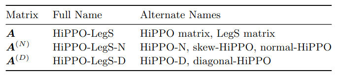
- $A$: HiPPO-LegS
- $A^{(N)}$: Normal / diagonal plus low-rank form
- $A^{(D)}$: diagonal matrix of DPLR / Eigenvalues of $A^{(N)}$
DSS paper made the surprising empirical observation that simply removing the low-rank portion of the DPLR form of the HiPPO-LegS matrix results in a diagonal matrix that performs comparably to the original S4 method. DSS initialization is $A^{(D)}$
Problems of DSS
- The strongest version of DSS computes the SSM with a complex-valued softmax that complicates the algorithm. The algorithm is less efficient than S4.
- DSS and S4 differ in several auxiliary aspects of parameterizing SSMs. This makes it more difficult to isolate the core effects of diagonal $A$ versus DPLR $A$.
- DSS relies on initializing the state matrix to a particular approximation of S4’s HiPPO matrix.
S4D
S4D, a simple method outlined by S4 for computing diagonal instead of DPLR matrices, which is based on Vandermonde matrix multiplication and is even simpler and more efficient than the DSS.
The new mathematical analysis of DSS’s initialization, showing that the diagonal approximation of the original HiPPO matrix surprisingly produces the same dynamics as S4 when the state size goes to infinity. We propose even simpler variants of diagonal SSMs using different initializations of the state matrix (see paper Section 4)
Discretization
Bilinear (used by S4)
\[\begin{align} \bar{A} &= (I - \Delta/2A)^{-1}(I + \Delta/2A) \\ \bar{B} &= (I - \Delta/2A)^{-1} \cdot \Delta B \end{align}\]ZOH (used by LMU and DSS)
\[\begin{align} \bar{A} &= \exp(\Delta A) \\ \bar{B} &= (\Delta A)^{-1}(\exp(\Delta \cdot A) - I) \cdot \Delta B \end{align}\]The discrete-time SSM output is:
\[y = u * \bar{K}\]where $\bar{K} = ( C\bar{B}, C\bar{A}\bar{B}, …, C\bar{A}^{L-1}\bar{B} )$
Convolution Kernel
The main computational difficulty of the original S4 model is computing the convolution kernel $\bar{K}$.
When $A$ is diagonal, the computation is nearly trivial:
\[\bar{K}_{\ell} = \sum_{n=0}^{N-1} c_n \bar{A}_n^{\ell} \bar{B}_n \quad \Rightarrow \quad \bar{K} = (\bar{B}^T \circ C) \cdot \mathcal{V}_{\ell}(\bar{A})\]where
- \(\mathcal{V}_{\ell}(A)_{n,\ell} = A_n^{\ell}\) is Vandermonde matrix
- $\circ$ is Hadamard product
- $\cdot$ is matrix multiplication
Or equivalently:
\[\bar{K} = \begin{bmatrix} \bar{B}_0C_0 & \cdots & \bar{B}_{N-1}C_{N-1} \end{bmatrix} \begin{bmatrix} 1 & \bar{A}_0 & \bar{A}_0^2 & \cdots & \bar{A}_0^{L-1} \\ 1 & \bar{A}_1 & \bar{A}_1^2 & \cdots & \bar{A}_1^{L-1} \\ \vdots & \vdots & \vdots & \ddots & \vdots \\ 1 & \bar{A}_{N-1} & \bar{A}_{N-1}^2 & \cdots & \bar{A}_{N-1}^{L-1} \end{bmatrix}\]Complexity
- The naive way to compute $\bar{K}_l$ requires materializing the Vandermonde matrix and requires $O(NL)$ time and space
- The optimal way to compute $\bar{K}_l$ only requires $O(N + L)$ operations and $O(N + L)$ space
- On GPU, the optimal way to compute $\bar{K}_l$ is to compute with
- $O(NL)$ operations
- $O(N + L)$ space, NOT materializing the Vandermonde matrix
Parameterization
Parameterization of $A$
If A has any eigenvalues with positive real part, $K(t) = Ce^{tA}B$ blows up to $\infty$ as $t to \infty$.
To force the real part of $A$ to be negative, one could use a technique call “left-half plane condition” in classic control: parameterize the real part of $A$ inside a negative exponential,
\[A = -\exp(A_{Re}) + i \cdot A_{Im}\]In fact, any one-side bounded function, such as -ReLU or -softplus, can be used to force $A$ to have negative real part.
Parameterization of $B,C$
$\bar{K}$ depends only on element-wise product $B \circ C$. Therefore, we can
- Directly parametrize the product as $W$
- Retain independent $B,C$, but freezing $B=1$ while training only $C$
- $C$ Can be randomly initialized with standard derivation 1
- This is different from typical DL initialization, which scale with dimension $N^{1/2}$
Conjugate Symmetry
We ultimately care about sequence transformation over real number $u(t)$ with real SSM $A$.
However, to diagonalize $A$, we need to look into complex SSM, since a broader set of real matrices can be diagonalized over the complex field.
Background on Linear Algebra
- Fundamental Theorem of Algebra
- Every non-zero, single-variable, degree $n$ polynomial with complex coefficients has exactly $n$ complex roots, when counted with multiplicity
- This guarantees that any characteristic polynomial of a matrix, has a solution in the complex field
- When the characteristic polynomial has distinct roots (eigenvalues), it is diagonalizable over the complex field
- When the characteristic polynomial has repeated root, it might be non-diagonalizable
- Algebraic multiplicity: multiplicity of an eigenvalue
- Geometric multiplicity: maximum number of linearly independent eigenvectors associated with an eigenvalue
- When algebraic multiplicity = geometric multiplicity for each of eigenvalue, the matrix is diagonalizable, otherwise the matrix is non-diagonalizable
- When a real matrix is diagonalized over the complex field, it can have
- Real eigenvalues
- Complex eigenvalues in conjugate pairs
Given the resulting diagonal parameters / eigenvalues always occur in conjugate pairs, we can throw out half of the parameters and implicitly add them back when computing $\bar{K}$ using Vandermonde matrix.
To parameterize a real SSM of state size $N$, we can
- Parameterize a complex SSM of state size $\frac{N}{2}$
- Implicitly add back the conjugate pairs of the parameters
- Implemented as real part $\times 2$, see S4D numpy implementation below
- When computing $K$ from Vandermonde matrix, the $N$-dim diagonal will collapse into $1$-dim in the matrix multiplication, leaving only the broadcasting length $L$ (see Convolution Kernel Section above)
S4D
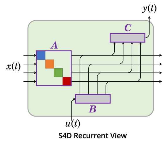
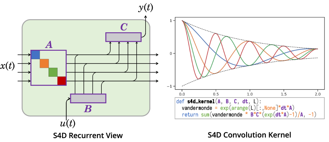
Visualization of S4D compute
- The diagonal structure allows transformation on $x(t)$ to be viewed as a collection of independently updated 1-dimensional SSMs
- Colors denote independent 1-D SSMs
- Purple denotes trainable parameters
The S4D method is very straightforward to implement:
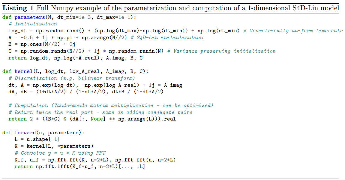
Comments over the numpy implementation
- Initialization of $\Delta$ and other components of the overall neural network architecture are the same as in S4 and DSS
- Size of complex SSM is half of the state size $N$:
N // 2 1jrepresent imaginary part- The powering up $A$ in Vandermonde matrix is implement different in practice (using exponential of $A$; for details, see repo)
- The “implicitly add back the conjugate pairs”:
K = 2 * ((B*C) @ (dA[:, None] ** np.arange(L))).real
Parameterization choices for Structured SSMs
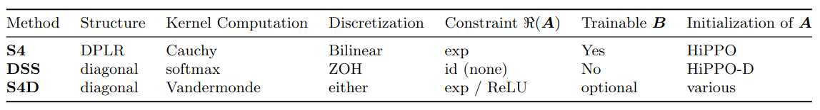
Output of S4D would be exactly the same as masking out the low-rank component of S4’s DPLR representation. Therefore, comparing S4D vs S4 is a comparison of diagonal vs. DPLR representations of $A$ while controlling all other factors.
S4D disentangles the discretization method from the kernel computation, whereas previous methods required a specific discretization.
Initialization of Diagonal State Matrices $A$
Expressivity and Limitations of Diagonal SSMs
Proposition 2
The set $D \subset \mathbb{C}^{N \times N}$ of diagonalizable matrices is dense in $\mathbb{C}^{N \times N}$, and has full measure (i.e. its complement has measure 0).
Explanation
$D$ is dense in $\mathbb{C}^{N \times N}$ means that every matrix in $\mathbb{C}^{N \times N}$ is either diagonalizable or can be approximated arbitrarily closely by diagonalizable matrices. In other words, for every non-diagonalizable matrix, there exists a sequence of diagonalizable matrices that converges to it.
Having full measure means that the set of diagonalizable matrices takes up almost the entire space of $\mathbb{C}^{N \times N}$. A set having full measure implies that the subset of non-diagonalizable matrices is so small that, for practical purposes, it can be considered negligible (it has measure zero).
Therefore, Proposition 2 is equivalent to saying (almost) all SSMs are equivalent to a diagonal SSM.
State Space Transformation
Any state-space transformation of the form $(V^{-1}AV,V^{-1}B,CV)$ is exactly equivalent to the original state-space $(A,B,C)$.
Implication: if you can find a matrix $V$ that diagonalizes $A$, you can represent the original system by a diagonal system without changing its behavior or properties, reinforcing diagonal SSM can represent almost all SSMs.
Limitations
The Proposition 2 is about expressivity: it tells us such diagonal SSM exist without telling us how to find it, nor does it guarantee strong performance of a trained model after optimization.
Previous works shows that parameterizing $A$ as a dense real matrix or diagonal complex matrix, performs poorly if randomly initialized.
The Proposition 2 also does not account for numerical stability, which is why DPLR in S4 is proposed (Lemma 3.2).
The open question is: which diagonal state matrices $A$ are effective?
- HiPPO-LegS?
- Approximation of HiPPO-LegS?
- Other?
S4D-LegS
Recall the convolutional kernel of SSM can be written as linear combination of basis kernel:
\[K(t) = \sum_{n=1}^{N-1} C_nK_n(t)\]where $K_n(t) = e_n^\top e^{tA} B$. The basis kernel only involves $A,B$ and can be written as $K_{A,B}(t)$
Theorem 3
Warning: please double check the S4’s code. It appears that the paper’s notation of $A^{(N)}$ should represent $N$-dim, but is overloaded with HiPPO-N matrix. This $A^{(N)}$ should be $A^{(D)}$ matrix with state dimension $N$. So I used lower case $n$ below.
Consider $A = A^{(n)} - P P^{\top}$ be DPLR representation of HiPPO-LegS or S4-LegS, where $A^{(n)}$ is a diagonal matrix and $n$ is number of state dimension. Let $K_{A,B}(t)$ be basis kernel. As the state size $n \to \infty$, the diagonal SSM basis converge to DPLR SSM basis:
\[K_{A^{(n)},B/2}(t) \to K_{A,B}(t)\]Theorem 3 explains why S4D-LegS performed quite close to S4-LegS: S4D-LegS is a noisy approximation of S4-LegS.
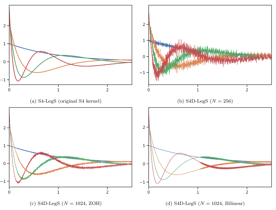
Visualization of Theorem 3
- Plot (a): The particular $(A, B)$ matrix chosen in S4 results in smooth basis functions $e^{tA}B$ with a closed form formula in terms of Legendre polynomials. By the HiPPO theory, convolving against these functions has a mathematical interpretation as orthogonalizing against an exponentially-decaying measure.
- Plot (b,c): By special properties of this state matrix, removing the low-rank term of its DPLR/NPLR representation produces the same basis functions as $n \to \infty$, explaining the empirical effectiveness of DSS.
- Plot (d): The bilinear transform smooths out the kernel to exactly match S4-LegS as $n$ grows.
S4D-Inv
Following a set of analysis and conjecture over the eigenvalues of HiPPO-LegS matrix $A$, the authors proposed S4D-Inv to use the following inverse-law diagonal matrix which closely approximates S4D-LegS:
\[A_{n} = -\frac{1}{2} + i \frac{N}{\pi} \left( \frac{N}{2n+1} -1 \right)\]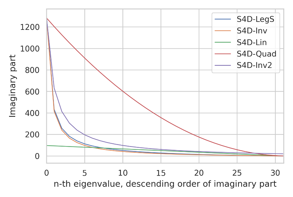
Eigenvalues for different S4D methods
- All S4D methods have eigenvalues $-\frac{1}{2} + \lambda_ni$.
- S4D-LegS (Blue): theoretically approximates dynamics of the original S4
- S4D-Inv (Orange): initialized with eigenvalues following an inverse law $\lambda_n \propto n^{-1}$, the plot shows its imaginary part approximate S4D-LegS
- The precise eigenvalues are important: other scaling laws with the same range perform empirically worse
- An inverse law with different constant (Purple)
- A quadratic law (Red)
- S4D-Lin (Green): A very different linear law based on Fourier frequencies also performs well
S4D-Lin
An even simpler scaling law for the imaginary parts that can be seen as an approximation of S4-FouT
The imaginary parts are simply the Fourier series frequencies (i.e. matches the diagonal part of the DPLR form of S4-FouT).
S4D-Lin basis $e^{tA}B$, which are simply damped Fourier basis functions.
General Diagonal SSM Basis Functions
The overall guiding principles for the diagonal state matrix A are
- The real part of $A_n$
- Controls the decay rate of the function
- $A_n = -\frac{1}{2}$ is a good default that bounds the basis functions by the envelope $e^{-t/2}$
- The imaginary part of $A_n$
- Controls the oscillating frequencies of the basis function
- Critically, these oscillating frequencies should be spread out, which explains why random initializations of $A$ do not perform well
- S4D-Inv and S4D-Lin use simple asymptotics for these imaginary components that provide interpretable bases
The authors believe that alternative initializations that have different mathematical interpretations may exist, which is an interesting question for future work.
Experiments
Sequential Benchmark Datasets
- Sequential CIFAR (sCIFAR)
- Length 1024 / 10-way classification
- BIDMC Vital Signs
- EKG and PPG signals of length 4000
- Predict respiratory rate (RR), heart rate (HR), and blood oxygen saturation (SpO2)
- Speech Commands (SC)
- 1-second raw audio / 16KHz / 35-way spoken word classification
Findings
- Computing the model with a softmax instead of Vandermonde product does not make much difference
- Training B is consistently slightly better
- Different discretizations do not make a noticeable difference
- Unrestricting the real part of A may be slightly better
For details, see paper’s [Table 2]
S4D Initialization Ablations
Findings: very simple changes that largely preserve the structure of the diagonal eigenvalues all degrade performance
For details, see paper’s [Table 3-a]
S4D vs S4
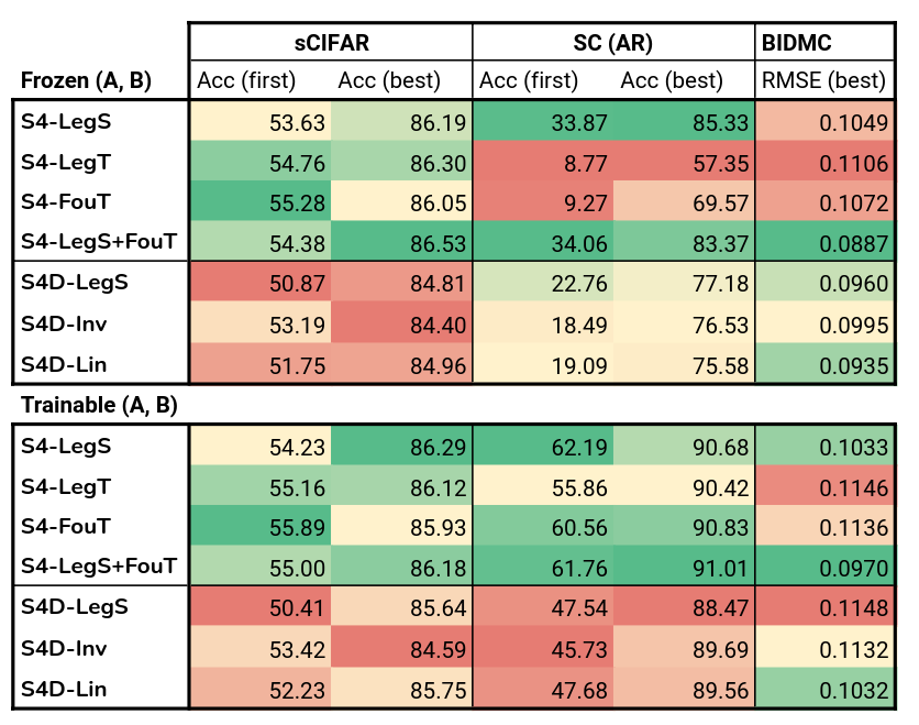
Findings
- Freezing vs training $A,B$
- Similar on sCIFAR and BIDMC
- Substantially worse on SC
- Hypothesize
- $\Delta$ is poorly initialized for SC, s.t. the models do not have context over the entire sequence
- Evidence: finite window methods S4-LegT and S4-FouT suffer the most when $A$ is frozen
- S4 vs S4D
- S4 often performs slightly better than S4D throughout the entire training curve
- Note that this is not a consequence of having more parameters
- Long Range Arena
- S4D variants are highly competitive on all datasets except Path-X
- S4D outperform S4 some benchmarks
- On average, S4D-LegS and S4D-Inv is competitive to S4 and significantly outperforms Transformer